Data Quality on Read

A Practical Guide to Mask-Based Data Profiling

Andrew Morgan

First Edition — 2026

Copyright

Data Quality on Read: A Practical Guide to Mask-Based Data Profiling

© 2026 Andrew Morgan

This work is licensed under the Creative Commons Attribution 4.0 International License (CC BY 4.0).

You are free to:

• Share — copy and redistribute the material in any medium or format
• Adapt — remix, transform, and build upon the material for any purpose, including commercially

Under the following terms:

• Attribution — You must give appropriate credit, provide a link to the license, and indicate if changes were made. You may do so in any reasonable manner, but not in any way that suggests the licensor endorses you or your use.

Full license text: creativecommons.org/licenses/by/4.0

Author: Andrew Morgan
Publisher: Andrew Morgan
First edition: 2026

Tools: dataradar.co.uk · github.com/minkymorgan/bytefreq
Source: github.com/minkymorgan/DataQualityOnRead
Contact: andrew@gamakon.ai

Foreword

Every organisation that works with data eventually discovers the same uncomfortable truth: the data is not what the documentation says it is. The specification describes an ideal. The file contains reality. The gap between them is where projects stall, budgets overrun, and decisions go wrong.

In nearly two decades of building data platforms — across financial services, government, telecoms, and open data — I have seen this gap consume more time, money, and goodwill than any other single problem in data engineering. Not because the problem is hard to understand, but because the tools for discovering it have historically been slow, expensive, and assumption-heavy. You needed to know what you were looking for before you could look for it.

Mask-based profiling inverts that assumption. It asks no questions about the data. It makes no assumptions about what the data should contain. It simply translates every value into its structural fingerprint and counts the results. The dominant patterns tell you what the data is. The rare patterns tell you what has gone wrong. The technique is mechanical, deterministic, and fast — and it works on any data, in any language, at any scale.

This book describes the technique, the architecture that surrounds it, and the open-source tools that implement it. It is written for practitioners: data engineers, analysts, and anyone who has ever opened a file and wondered what they were looking at. The ideas are simple. The implementation is straightforward. The impact, in my experience, is transformative.

I hope you find it useful.

Andrew Morgan February 2026

Introduction

In 2007, while working on a data migration for a financial services client, we received a file that was described as containing customer addresses. The specification said the fields were fixed-width, ASCII-encoded, with UK postcodes in column 47. When we loaded the file and profiled it, we discovered that column 47 contained a mixture of valid postcodes, phone numbers, the string "N/A" repeated 11,000 times, and — in one memorable case — what appeared to be someone's lunch order.

The specification was wrong. Or rather, the specification described what the data should look like, and the file contained what the data actually looked like. These are not the same thing, and the gap between them is where data quality lives.

This experience, repeated in various forms across financial services, telecoms, government, and open data projects over nearly two decades, led to the development of a simple but surprisingly powerful technique: mask-based data profiling. The idea is straightforward. Take every character in a data field and translate it to its character class — uppercase letters become A, lowercase become a, digits become 9, and everything else (punctuation, spaces, symbols) stays as it is. The result is a structural fingerprint of the value, a mask, that strips away the content and reveals the shape of the data underneath.

When you profile a column by counting the frequency of each mask, patterns emerge immediately. The dominant masks tell you what the data is supposed to look like. The rare masks — the long tail — tell you where the problems are hiding. No regex, no schema, no assumptions about the data required. Just a mechanical translation that lets the structure speak for itself.

This book describes that technique, the architecture around it, and the tools that implement it. The technique itself is called Data Quality on Read (DQOR), a deliberate parallel to the "Schema on Read" principle that underpins modern data lake architectures. The core idea is the same in both cases: accept raw data as-is, defer processing until the moment of consumption, and never overwrite the original. In the schema case, you defer structural interpretation. In the quality case, you defer profiling, validation, and remediation. The benefits are the same: agility, provenance, and the ability to reprocess history when your understanding improves.

The tools are bytefreq, an open-source command-line profiler now implemented in Rust, and DataRadar, a browser-based profiling tool that runs entirely client-side using WebAssembly. Both implement DQOR from the ground up, and both are free to use.

The book is structured in three parts. Part I sets out the problem: why data quality is hard, and why the traditional approaches — schema validation, statistical profiling, regex-based checks — leave gaps that mask-based profiling can fill. Part II introduces the technique in detail: masks, grain levels, Unicode handling, population analysis, error codes, and treatment functions. Part III describes the architecture that ties it all together: the flat enhanced format (a trick borrowed from Hadoop-era feature stores), and the tools that implement it at different scales.

The intended audience is anyone who works with data they did not create: data engineers, analysts, scientists, and the growing number of people who find themselves responsible for data quality without having chosen it as a career. The technique is simple enough to prototype in a single line of sed, and powerful enough to run in production at enterprise scale. We will cover the full range.

Discovery Before Exploration

Before you profile the values in a field, you need to know what fields exist and how populated they are. This sounds obvious. It is obvious. And yet the most common mistake in data quality work is to dive straight into field-level analysis — examining the values in a column — without first understanding the shape of the dataset as a whole. Structure discovery comes before content exploration. Always.

For tabular data — CSV files, fixed-width extracts, pipe-delimited feeds — this means counting non-null values per column. If a dataset has 55 columns but only 20 of them are more than 50% populated, that fact alone reshapes your entire profiling strategy. You do not need to know what is in the other 35 columns yet. You need to know they are mostly empty. That knowledge takes seconds to acquire and saves hours of misdirected effort.

For nested data — JSON, XML, hierarchical formats — the same principle applies, but the discovery step is different. You walk the structure to find every field path, then count how many records contain each path. A JSON feed might have 200 distinct field paths, but any given record might populate only 40 of them. A field that appears in 10% of records tells you something important before you have looked at a single value. A field that appears in 100% of records tells you something different. The population profile across all paths is the first thing you need, and the last thing most people think to check.

Think of it as a census before a survey. The census maps the territory: what exists, where it is, how much of it there is. The survey examines individual items in detail. Running the survey without the census means you do not know what you are missing, what you are over-sampling, or where your effort is best spent. The field population profile is the map. Profile without it and you are navigating blind.

This principle prevents wasted effort in both directions. Profiling a field that is 99% empty is rarely the best use of your time — you will generate a mask frequency table dominated by a single empty-value pattern and learn almost nothing. Conversely, discovering that a field described as "mandatory" in the specification is only 45% populated is itself a significant data quality finding — and you found it in the discovery phase, before spending any time on content analysis. Some of the most valuable insights come from the map, not from the territory it describes.

The worked examples in this book follow this principle explicitly. Each begins with a structure discovery phase — field counts, population rates, structural metadata — before moving to field-by-field mask analysis. This is not a stylistic choice. It is the method. Discovery before exploration, every time.

Data Quality Without Borders

The world's largest generators and consumers of data are in the public sector. Central, regional, and local governments manage millions of data transfers across ministerial boundaries every day. This separation of concerns makes government the single largest environment where Data Quality on Read is most urgently needed.

The stakes are high. "Single view of citizen" systems help governments deliver better services and ensure people do not fall between the cracks. But building these views requires integrating data from systems that were never designed to talk to each other, encoded in formats nobody fully documented. And because the data is personally identifiable, access to view raw records is rightly restricted — making data quality work uniquely difficult. You need to understand structure and quality without seeing content. This is where mask-based profiling shines: a mask reveals the shape of the data without exposing whose data it is.

The 33 languages in DataRadar's first tier of localisation — from English and French to Amharic, Hausa, Swahili, Tamil, Nepali, and Chinese — cover approximately 5.5 billion citizens. Data quality tools have historically supported only English interfaces and Latin-script datasets. A civil servant in Addis Ababa profiling census data in Amharic, or a local government analyst in Lagos working with Hausa-language records, had no tools built for them. DataRadar and bytefreq are.

All citizens deserve effective government services, and data quality is a prerequisite for delivering them. Multilingual, privacy-first, zero-install tools that work across scripts, languages, and borders — that is the ambition.

From Files to Services

The techniques in this book can profile a single file in seconds. But the real prize is bigger than files.

Consider a government department that receives data from dozens of external collectors — local councils, NHS trusts, schools, partner agencies — and publishes onward to downstream consumers. How does a Chief Data Officer know whether the department is producing good quality data? How does a CTO assure the service, not just individual datasets?

The answer is to treat data quality profiling as infrastructure, not as a one-off activity. The building blocks described in this book — mask-based profiling, the flat enhanced format, population analysis, assertion rules — are designed to assemble into a monitoring architecture that can assure an entire data service.

The pattern has two sides.

Exit checks run at the point of production. Before a department publishes a data feed, the profiling engine runs against the output and generates a quality report — mask distributions, population rates, character encoding composition, assertion rule results. This report is stored as a timestamped fact record. Over weeks and months, a timeseries builds up: a continuous measurement of what the department is actually shipping.

Entrance checks run at the point of consumption. When a downstream system receives a data feed, the same profiling engine runs against the input. The entrance report is compared against the expected baseline (derived from the exit checks or from an agreed specification). Deviations are flagged. New masks appearing, population rates dropping, encoding shifts — all are detected automatically, before the data enters the consumer's pipeline.

Between these two checkpoints, something powerful emerges: line of sight. When a downstream system encounters a quality issue, the entrance check report traces it back to the feed. The feed's exit check report traces it back to the collector. The timeseries shows when the problem started. Connected to lineage tools that track data flow across systems, this creates an automated root cause analysis — not "something is wrong somewhere" but "this specific field in this specific feed from this specific collector started producing a new mask pattern on this date, and the downstream impact is quantifiable."

That quantification matters. When you can say "Department X's data collection issues caused 2,000 downstream failures last quarter, costing an estimated £Y million in rework, delayed decisions, and incorrect outputs," the conversation changes. Quality stops being an abstract concern and becomes a line item. The timeseries is the measuring stick that makes consistent performance conversations possible — not blame, but evidence.

This reframes the purpose of data quality. The traditional question is: "Is this data fit for purpose?" — meaning, can the immediate consumer use it? The better question is: "Is this data fit for the journey?" Data rarely has one consumer. A dataset collected by a local council may pass through a regional aggregator, a central government platform, a statistical publication pipeline, and a public API before reaching its final consumers. Quality at the point of collection is not enough if the data degrades, is misinterpreted, or hits structural incompatibilities at any stage of that journey. Fit for the journey means the data carries enough structural metadata — masks, population profiles, assertion results — to be understood and validated at every stage, by every hand it passes through.

The profiling reports described in this book — both the DQ mask frequency tables and the CP character profiling reports — are the raw telemetry for this monitoring architecture. They are structured, machine-readable, and designed to be stored and queried as fact tables. The technical implementation — time-partitioned directories, DuckDB queries, KPI dashboards — is covered in the Quality Monitoring chapter in Part III.

The tools in Part III are the building blocks. The architecture they enable is a data quality assurance service: continuous, measurable, and accountable.

Let's begin.

Why Data Quality Still Breaks Things

There is a widely cited statistic that poor data quality costs organisations between 15 and 25 percent of revenue. The number has been repeated so often that it has become background noise, the kind of thing people nod at in presentations and then promptly ignore when scoping their next project. The reason it persists, despite everyone knowing about it, is structural: most data quality problems are invisible until they cause a failure downstream, and by then the cost of remediation is orders of magnitude higher than the cost of early detection.

Consider a simple example. A retail company receives a daily feed of product catalogue updates from a supplier. The feed is a CSV file, delivered via SFTP, containing product codes, descriptions, prices, and stock levels. The specification says prices are in GBP, formatted as decimal numbers with two decimal places. For six months the feed arrives on time, the prices parse correctly, and everyone is happy. Then one Monday the supplier's system is upgraded, and the price field starts arriving with a currency symbol prefix — £12.99 instead of 12.99. The downstream pricing engine, which casts the field to a numeric type, throws a parse error. The product catalogue goes stale. Customer-facing prices are wrong for four hours until someone notices and writes a hotfix.

The fix takes ten minutes. The investigation takes two hours. The post-incident review takes half a day. The customer complaints take a week to resolve. The root cause was a single character in a single field, and the total cost — in engineering time, reputational damage, and operational disruption — was wildly disproportionate to the simplicity of the underlying issue.

This pattern repeats across every industry that depends on data received from sources it does not control. The specific failures vary — date formats flip between DD/MM/YYYY and MM/DD/YYYY, encoding shifts from UTF-8 to Latin-1, a column that was always numeric starts containing the string NULL instead of an actual null — but the shape of the problem is always the same. Data that was assumed to be clean turns out not to be, and the assumption is only tested at the point of failure.

The Read Problem

Most data quality tooling is designed around the assumption that you control the data pipeline end to end. Schema validation at the point of entry, constraint enforcement in the database, type checking in the application layer — these are all "quality on write" techniques, and they work well when you are the author of the data. The difficulty arises when you are the reader rather than the writer.

In modern data architectures, the proportion of data that arrives from sources you do not control is substantial and growing. Third-party feeds, partner integrations, open data portals, scraped web content, legacy system exports, IoT sensor streams, and API responses from services maintained by other teams — all of these represent data that was created according to someone else's assumptions, documented (if at all) according to someone else's standards, and delivered with whatever level of quality the source system happened to produce that day.

You cannot fix the source. In many cases you cannot even influence it. What you can do is understand what you have received, quickly and cheaply, before you attempt to use it. That understanding — structural, not semantic — is the domain of Data Quality on Read.

What Goes Wrong

In working with data platforms across financial services, telecoms, government, and open data projects, we have seen the same categories of data quality failure appear repeatedly. They are worth enumerating because they inform the design of the profiling techniques that follow.

Format inconsistency is the most common. A date column contains values in three or four different formats — 2024-01-15, 15/01/2024, Jan 15 2024, and occasionally just 2024 — because the upstream system aggregated data from multiple sources without normalising it. A phone number column mixes UK mobile (07700 900123), international (+44 7700 900123), US ((555) 123-4567), and free-text entries like "ask for Dave". Each of these is individually valid; the problem is that they coexist in the same column with no indicator of which format applies to which record.

Encoding corruption is subtler and often goes undetected for longer. A file that was encoded in Latin-1 is read as UTF-8, producing garbled characters in names and addresses. A BOM marker at the start of a CSV causes the first column header to parse incorrectly. Control characters — tabs, carriage returns, null bytes — appear in fields that should contain only printable text, breaking downstream parsers that assumed simple delimited input.

Structural drift happens when the shape of the data changes over time without corresponding updates to the documentation or the downstream systems that consume it. A new column is added to a feed, shifting all subsequent field positions. An optional field starts being populated where it was previously always empty, triggering unexpected code paths. A field that was always a single value starts containing comma-separated lists.

Placeholder abuse is endemic. The strings N/A, NULL, none, n/a, -, TBC, unknown, test, and the empty string all appear in production data as substitutes for missing values, each encoded differently, each requiring different handling, and none of them matching the expected format of the field they occupy. In one government dataset we profiled, the placeholder REDACTED appeared in the postcode field of 3% of records, which was useful to know before attempting geocoding.

Population shifts are the hardest to detect without profiling. The data looks structurally correct — all the fields parse, all the types are right — but the distribution has changed. A column that previously had 99.5% population now has 15% nulls because an upstream collection process was turned off. A field that used to contain 8 distinct values now contains 47, because a system migration expanded the code set without updating the documentation.

None of these problems are exotic. They are the ordinary, everyday reality of working with data that someone else created. The question is not whether they exist in your data — they almost certainly do — but whether you have a systematic way of finding them before they cause harm.

The Limits of Traditional Approaches

Before introducing mask-based profiling, it is worth understanding why the existing approaches leave gaps. Not because they are bad — many of them are excellent at what they do — but because they share a common assumption that limits their applicability to the "quality on read" problem.

Schema Validation

The most established approach to data quality is schema validation: define the expected types, formats, and constraints for each field, then reject or flag records that do not conform. This is the approach used by database constraints, JSON Schema, XML Schema (XSD), Avro, Protobuf, and a host of other technologies. It works well in systems where you control the schema and the data is produced by software that respects it.

The limitation is that schema validation requires you to know what the data should look like before you receive it. When you are exploring a new dataset — a third-party feed you have never seen before, an open data portal with sparse documentation, or a legacy system export where the specification was written ten years ago and has not been updated since — the schema is precisely the thing you are trying to discover. Validating against an assumed schema at this stage risks either rejecting valid data that does not match your assumptions, or accepting invalid data that happens to pass your checks by coincidence.

There is also the problem of data that is "technically valid" but semantically broken. A date field containing 0000-00-00 will pass a format check for YYYY-MM-DD but is clearly not a real date. A numeric field containing 999999 will pass a type check but may be a sentinel value meaning "not applicable." Schema validation catches structural violations but tells you nothing about whether the values themselves make sense.

Statistical Profiling

Tools like Great Expectations, dbt tests, and pandas-profiling take a different approach: compute summary statistics for each column (null counts, min/max values, cardinality, distributions, standard deviations) and flag deviations from expected ranges. This is useful for ongoing monitoring of data pipelines where you have a baseline to compare against, and it catches population-level issues (sudden spikes in nulls, unexpected changes in cardinality) that schema validation misses.

The limitation is that aggregate statistics hide structural detail. A column with 99% valid email addresses and 1% phone numbers will report a cardinality, a null rate, and a string length distribution that all look reasonable. The phone numbers — wrong data in the wrong field — will not appear as outliers in any statistical measure because they are structurally similar to emails in terms of length and character composition. You need to see the patterns to spot the problem, and summary statistics do not show patterns.

Statistical methods also require a baseline: they tell you that something has changed, but not what the data looks like in the first place. For initial exploration of an unfamiliar dataset, they give you numbers without context.

Regex-Based Validation

Regular expressions allow precise format validation: a UK postcode matches [A-Z]{1,2}[0-9R][0-9A-Z]? [0-9][ABD-HJLNP-UW-Z]{2}, an email matches a well-known (and notoriously complex) pattern, a date matches \d{4}-\d{2}-\d{2}. When you know exactly what formats to expect, regex validation is powerful and precise.

The limitation is combinatorial. Each expected format requires its own expression. A phone number column that contains UK mobiles, UK landlines, international numbers with country codes, and US-formatted numbers needs at least four regex patterns — and that is before you account for variations in spacing, punctuation, and prefix formatting. For every new format you discover, you write another regex. For every field in every dataset, you maintain a library of patterns. The approach does not scale to exploratory work where you do not yet know what formats exist.

More fundamentally, regex validation is a confirmation technique: it confirms that data matches a pattern you already know about. It does not help you discover what patterns exist in data you have never seen before. Discovery requires a different tool.

What They All Share

All three approaches — schema validation, statistical profiling, and regex-based validation — share a common assumption: you already know what the data should look like. They are verification techniques, designed to confirm expectations. When those expectations are correct and the data is well-understood, they work beautifully.

The gap they leave is in discovery: the initial exploration of unfamiliar data, where you have no schema, no baseline statistics, and no library of expected formats. You need something that will show you what the data does look like, without requiring you to tell it what to look for. That is the role of mask-based profiling.

Schema on Read, Quality on Read

The idea of deferring structural interpretation until the point of consumption is well established in data architecture. In the Hadoop era, it acquired a name — Schema on Read — and it changed how large-scale data platforms were designed. Rather than enforcing a rigid schema at the point of ingest (Schema on Write, the relational database approach), data lakes accept raw data in whatever format it arrives, store it cheaply, and apply structural interpretation only when a consumer reads the data for a specific purpose.

The benefits of Schema on Read are widely understood. Raw data is preserved in its original form, providing provenance and auditability. Multiple consumers can apply different schemas to the same underlying data, supporting different use cases without duplicating pipelines. When schemas change — and they always change — historical data does not need to be reprocessed, because the raw material is still there. The trade-off is that consumers bear the cost of interpretation, but in practice this cost is modest compared to the flexibility gained.

Data Quality on Read (DQOR) applies exactly the same principle to data quality processing. Instead of cleansing, validating, enriching, and remediating data at the point of ingest — which requires perfect upfront knowledge of the data, slows pipeline velocity, and risks overwriting original values with incorrect corrections — DQOR defers all quality processing until the moment the data is actually consumed.

The core workflow is simple:

1. Ingest raw data as fast as possible, preserving it exactly as received.
2. At read time, profile the data to discover its structural characteristics.
3. Generate quality metadata (masks, assertions, suggested treatments) alongside the raw values.
4. Let downstream consumers choose which treatments to apply — or to ignore them entirely and work with the original.

The raw data is never overwritten. The quality metadata is never mandated. Consumers see both the original value and the profiler's assessment of it, and they make their own decisions about what to trust. This is a fundamental design choice: suggestions, never mandates.

Why This Matters

There are several practical reasons why deferring quality processing to read time is advantageous, particularly for data received from external sources.

First, it preserves the original data as an immutable audit trail. In regulated industries (financial services, healthcare, government), the ability to trace a derived value back to the exact bytes that were received from the source system is not a convenience — it is a compliance requirement. DQOR provides this by construction, because the raw data is never modified.

Second, it accommodates imperfect knowledge. When you first receive a new data feed, you rarely understand it fully. The documentation may be incomplete, the specification may be out of date, and the actual data may contain patterns that nobody anticipated. If you apply quality rules at ingest time based on incomplete understanding, you risk discarding or corrupting valid data. By deferring quality processing, you give yourself time to learn the data before committing to a treatment strategy — and when your understanding improves, you can reprocess the history without re-ingesting it.

Third, it supports multiple consumers with different quality requirements. A data science team exploring patterns in raw sensor data may want the original values, noise and all. A reporting team feeding a customer-facing dashboard may want aggressively cleaned and normalised data. A compliance team may want to see every record that was flagged as anomalous, with the raw value alongside the flag. DQOR supports all three from the same source, without separate pipelines.

Fourth, it decouples ingest velocity from quality processing. Data acquisition pipelines can focus on reliability and throughput — landing data on the platform as fast as the source can deliver it — without being slowed by the computational overhead of profiling, validation, and remediation. Quality processing happens later, on the consumer's schedule, using the consumer's compute budget. In streaming architectures, where latency matters, this decoupling is particularly valuable.

The Parallel With Feature Stores

For anyone who has worked with machine learning feature stores, the DQOR pattern will feel familiar. A feature store holds pre-computed features alongside the raw data they were derived from, so that model-serving pipelines can retrieve prediction-ready inputs without recomputing them at request time. The raw data is never discarded; the features are additive layers that sit alongside it.

DQOR follows the same structural logic. The raw value is preserved. Quality metadata — masks, assertions, suggested treatments — are generated as additional columns that sit alongside the raw value in the same row. Downstream consumers select the columns they need. Adding a new quality check or a new treatment is just adding another column; it never touches the original data, and it never requires reprocessing existing outputs.

The enhanced output is a nested record format — each field in the original data becomes a JSON object containing the raw value, its masks, and any inferred rules. The flat enhanced format takes this a step further: a flattened key-value pair schema, sourced from nested data (e.g. fieldname.raw, fieldname.HU, fieldname.Rules.is_numeric). Quality metadata travels with the data it describes — no joins, no lookups, no separate tables. We will return to the specific implementation of this pattern in Chapter 9.

Mask-Based Profiling

A mask, in the context of data profiling, is a transformation function applied to a string that generalises the value into a structural fingerprint. The transformation replaces every character with a symbol representing its character class, while preserving punctuation and whitespace. When a column of data is summarised by counting the frequency of each resulting mask — a process commonly called data profiling — it reveals the structural patterns hiding inside the data, quickly and without assumptions.

The basic translation is as follows:

• Uppercase letters (A–Z) are replaced with A
• Lowercase letters (a–z) are replaced with a
• Digits (0–9) are replaced with 9
• Everything else — punctuation, spaces, symbols — is left unchanged

It seems like a very simple transformation at first glance. To see why it is useful, consider applying it to a column of data that is documented as containing domain names. We expect values like nytimes.com. Applying the mask, we get:

   232  aaaa.aaa
   195  aaaaaaaaaa.aaa
   186  aaaaaa.aaa
   182  aaaaaaaa.aaa
   168  aaaaaaa.aaa
   167  aaaaaaaaaaaa.aaa
   167  aaaaa.aaa
   153  aaaaaaaaaaaaa.aaa

Very quickly, the mask reduces thousands of unique domain names down to a short list of structural patterns — all of which look like domain names, confirming our expectation. But what about the long tail? The rare masks that appear only a handful of times?

     2  AAA Aa
     1  a.99a.a
     1  9a9a.a

There is a mask — AAA Aa — that does not contain a dot, which we would expect in any domain name. This immediately stands out as structurally different from the rest. When we use the mask to retrieve the original values, we find the text BBC Monitoring — not a domain name at all, but a general descriptor that someone has used in a field designed for domain names. In re-reading the GDELT documentation we discover that this is not an error but a known special case, meaning when we use this field we must handle it. Perhaps we include a correction rule to swap the string for the valid domain www.monitor.bbc.co.uk, which is the actual source.

A second example, from real UK Companies House data, shows what happens when a field contains data from the wrong column entirely. The RegAddress.PostTown field — the registered office town — produces dozens of masks at LU grain. The dominant patterns are all legitimate town names: A (single words like READING, 84.2%), A A (two words like HEBDEN BRIDGE, 6.3%), and several hyphenated or abbreviated forms. But in the long tail:

Mask        Count   Example
A9 9A          14   EH47 8PG
9 A A          32   150 HOLYWOOD ROAD
9-9 A A        10   1-7 KING STREET
9A A            1   2ND FLOOR
9               2   20037

Postcodes in the town field. Street addresses in the town field. A US ZIP code. A floor number. The masks expose column misalignment that no town-name validation rule would detect — because EH47 8PG is a perfectly valid string, just in the wrong column. The mask A9 9A in a town field is diagnostic: towns do not have that structure, but postcodes do. (For the complete field-by-field analysis of this dataset, see the Worked Example: Profiling UK Companies House Data appendix.)

The idea we are introducing here is that a mask can be used as a key to retrieve records of a particular structural type from a particular field. Before we explore that idea further (it leads directly to the concept of masks as error codes, covered in Chapter 7), it is worth understanding the mechanics of the mask itself in more detail.

Why Masks Work

The power of mask-based profiling comes from a simple mathematical property: the mask function is a many-to-one mapping that dramatically reduces cardinality while preserving structural information. A column of ten million customer names might contain two million unique values, but after masking it might contain only a few hundred unique patterns. A column of phone numbers with a million unique values might collapse to a dozen structural formats.

This cardinality reduction is what makes manual inspection feasible. No human can review two million unique names, but anyone can scan a frequency table of two hundred masks and immediately identify the dominant patterns and the outliers. The mask strips away the content (the specific name, the specific number) and reveals the shape (the format, the structure, the encoding).

Consider a customer name column:

From the masks alone, without looking at the values, we can see: most records are capitalised names (Aaaa Aaaaa), some are in all-caps or all-lowercase (normalisation candidates), some contain apostrophes or hyphens (legitimate but structurally distinct), one is numeric (almost certainly an error — a customer ID in a name field), and one is a placeholder. The mask gives us a classification of structural types in a single pass.

A worked example from the French lobbyist registry illustrates this vividly. The first name field (dirigeants.prenom) produces four masks at LU grain:

Mask        Count   Example
Aa            697   Carole
Aa-Aa          50   Marc-Antoine
Aa Aa          11   Marie Christine
Aa_a            1   Ro!and

The first three are expected: simple names, hyphenated compounds (common in French), and space-separated compounds. The fourth is the standout: Aa_a — one record where Ro!and contains an exclamation mark where the letter l should be. The intended name is Roland, but a data entry error has replaced a letter with adjacent punctuation. No schema would catch this — the field is a valid string. No length check would catch it — six characters is reasonable. But the mask catches it instantly because ! is punctuation, not a letter, and the structural pattern is fundamentally different from every other value in the field. (For the full analysis, see the Worked Example: Profiling the French Lobbyist Registry appendix.)

Prototyping on the Command Line

One of the virtues of mask-based profiling is that it can be prototyped with standard Unix tools in a single line:

cat data.csv | gawk -F"\t" '{print $4}' | \
  sed "s/[0-9]/9/g; s/[a-z]/a/g; s/[A-Z]/A/g" | \
  sort | uniq -c | sort -r -n | head -20

This extracts column 4 from a tab-delimited file, applies the A/a/9 mask using sed, sorts the results, counts unique masks, and displays the top 20 by frequency. It runs in seconds on files with millions of rows, and the output is immediately interpretable. We open-sourced a more fully-featured version of this profiler — called bytefreq (short for byte frequencies) — originally written in awk, and later rewritten in Rust. The awk version is available for readers who want to understand the mechanics; the Rust version is what you would use in production. Both are discussed in Chapter 10.

The ability to prototype the technique in a one-liner is important not because the one-liner is a production tool, but because it demonstrates that the underlying idea is genuinely simple. There is no machine learning, no complex configuration, no training data. It is a mechanical character-by-character translation followed by a frequency count. The power comes not from the complexity of the method but from the interpretability of the output.

Grain, Scripts, and Character Classes

The basic A/a/9 mask described in the previous chapter works well for ASCII data and covers the majority of use cases in structured data profiling. But real-world data — particularly data sourced from open data portals, international organisations, and multilingual systems — contains characters that the simple ASCII mask cannot adequately describe. Accented characters, CJK ideographs, Arabic script, Devanagari, Cyrillic, Thai, Ethiopic, and increasingly emoji all appear in production datasets, and a profiler that treats them all as "other" is losing information.

This chapter introduces two extensions to the basic mask: grain levels, which control the resolution of the mask, and Unicode-aware character class translation, which extends masking across the full range of human writing systems.

High Grain and Low Grain

A high grain mask preserves the exact length and position of every character in the original value. Every character maps individually, so John Smith becomes Aaaa Aaaaa and Jane Doe becomes Aaaa Aaa. These are two different masks, because the strings have different lengths.

A low grain mask collapses consecutive runs of the same character class into a single symbol. Under low grain masking, John Smith becomes Aa Aa, and Jane Doe also becomes Aa Aa. The two values now share the same mask, because at the low grain level they have the same structure: a capitalised word followed by a space followed by another capitalised word.

The distinction matters because the two grain levels serve different purposes.

Low grain is the tool for discovery. When you first encounter an unfamiliar dataset and want to understand the structural families present in a column, low grain masking collapses millions of unique values into a handful of patterns. A name column that produces thousands of unique high grain masks (varying by name length) might produce only four or five low grain masks: Aa Aa (first name, last name), Aa A. Aa (with middle initial), Aa (single name), 9 (numeric — investigate), and A/A (placeholder). This immediate simplification makes the data comprehensible at a glance.

The effect is dramatic with non-Latin scripts. When profiling Japanese earthquake data from JMA, the hypocenter name field — containing kanji place names of varying length and composition — collapses entirely to a single mask at LU grain:

Mask    Count   Example
a          78   福島県会津
a_a         1   (compound name with punctuation)

78 of 79 values produce the same mask: a. Every CJK ideograph is classified as a lowercase letter (Unicode category Lo), and low grain collapses consecutive characters of the same class. A four-character name and an eight-character name are structurally identical at this grain. That one exception — a_a, a name containing a punctuation separator — stands out immediately. At HU grain, these 78 records would produce dozens of distinct masks varying by character count. At LU grain, you see the structural family at a glance. (See the Worked Example: Profiling JMA Earthquake Data appendix for the full analysis.)

High grain is the tool for precision. Once you have identified the structural families using low grain, you can drill into a specific family with high grain masking to see the exact formats. For a postcode column, low grain might tell you that most values match AA9 9AA (low grain: A9 9A). High grain will tell you that you have AA99 9AA, A99 9AA, A9 9AA, AA9 9AA, and AA9A 9AA — the five standard UK postcode formats — each with its own frequency, allowing you to verify completeness and detect anomalies.

A subtler example of when HU grain is needed comes from the French lobbyist registry. The title field (dirigeants.civilite) contains M (Monsieur) and MME (Madame). At LU grain, both collapse to A — a single mask covering all 760 values, suggesting perfect uniformity. At HU grain, M produces A and MME produces AAA, cleanly separating the two populations. The LU profile tells you the field is consistently alphabetic. The HU profile tells you there are exactly two formats and what they are. The choice of grain determines the question you are answering. (See the Worked Example: Profiling the French Lobbyist Registry appendix.)

The typical workflow is a two-pass approach: start with low grain to survey the landscape, then switch to high grain to examine specific areas of interest. This mirrors how experienced data engineers actually work — broad scan first, targeted investigation second — and the two grain levels formalise that workflow into the tool.

Unicode Character Classes

The original bytefreq implementation, written in awk and designed for ASCII data, mapped characters byte-by-byte. Each byte (0–255) was assigned a character class based on its position in the ASCII table, and the mapping was deterministic regardless of the encoding of the input. This had the pragmatic advantage of working consistently on any input — including binary data and files with mixed or unknown encodings — because it made no assumptions about what the bytes represented. It was, deliberately, a byte-level tool.

As the world has moved to Unicode, the byte-level approach needed extending. Modern datasets contain text in dozens of scripts, and a useful profiler needs to handle them without requiring language-specific configuration. The current implementations — both the Rust-based bytefreq CLI and the WebAssembly-based DataRadar browser tool — support Unicode-aware masking at two levels, which we call HU (High Unicode) and LU (Low Unicode), extending the high/low grain concept into the Unicode space.

Under Unicode-aware masking, the character class translation uses the Unicode General Category to determine how each character is mapped:

• Lu (Letter, uppercase) → A
• Ll (Letter, lowercase) → a
• Lt (Letter, titlecase) → A
• Lo (Letter, other — CJK ideographs, Arabic, Thai, etc.) → a
• Nd (Number, decimal digit) → 9
• Punctuation categories (Pc, Pd, Pe, Pf, Pi, Po, Ps) → kept as-is
• Symbol categories (Sc, Sk, Sm, So) → kept as-is
• Separator categories (Zs, Zl, Zp) → kept as-is

This means that a Chinese place name like 北京饭店 (Beijing Hotel) produces a mask of aaaa (four Lo characters, each mapped to a), an Arabic address produces a a a preserving the spaces between words, and an Icelandic name like Jökulsárlón produces Aaaaaaaaaa — preserving the capitalisation structure even though the accented characters are outside the basic ASCII range.

The practical benefit is that profiling works across scripts without configuration. When profiling a global places dataset containing names in Chinese, Thai, Arabic, Cyrillic, Devanagari, Ethiopic, and Latin scripts, the profiler does not need to be told which languages to expect. It uses the Unicode category of each character to generate masks that preserve structure, and the frequency analysis surfaces the dominant patterns regardless of script.

Script Detection

In addition to mask generation, both DataRadar and bytefreq perform automatic script detection per field, reporting the dominant scripts found in each column. This is implemented by examining the Unicode script property of each character and aggregating across all values in the field.

Script detection serves two purposes. First, it flags potential encoding issues: a column that is expected to contain Latin-script names but reports a significant minority of Cyrillic characters may have an encoding corruption (Cyrillic and Latin share visual forms for several characters, and mojibake — text decoded with the wrong character set — often manifests as unexpected script mixing). Second, it informs downstream processing: a column containing mixed Latin and Arabic text may need bidirectional text handling, which is worth knowing before it breaks a downstream rendering system.

Character Profiling

Character Profiling — CP mode — is a complementary technique to mask profiling. Where mask profiling translates each character to its class (A, a, 9) and counts the frequency of the resulting masks, CP mode counts the actual characters — the literal Unicode code points — present in a field. The question it answers is different: not "what structures exist in this data?" but "what characters actually appear in this data?"

This distinction is particularly revealing for non-Latin scripts. When profiling Japanese earthquake data from JMA (the Japan Meteorological Agency), CP mode revealed the presence of full-width digits (０, １, ２, ３ and so on) alongside standard ASCII digits (0, 1, 2, 3). At LU grain, both full-width and ASCII digits map to 9, so mask profiling alone cannot distinguish them — the masks are identical. CP mode surfaces the actual character inventory, making the mixing of digit forms immediately visible.

CP mode is equally powerful for detecting encoding anomalies. Consider a field that should contain French accented characters — é, è, ê, ç, à — but whose character inventory also includes Â, Ã, or the sequence ©. Those are the telltale signatures of mojibake: UTF-8 byte sequences that have been decoded as Latin-1 (or Windows-1252). The multi-byte UTF-8 encoding of é (0xC3 0xA9) becomes é when misinterpreted as two single-byte Latin-1 characters. The character inventory is the diagnostic — you do not need to write encoding-specific validation rules, because the wrong characters simply show up in the profile.

The practical workflow is straightforward: run mask profiling first to understand the structural patterns in your data, then run CP mode on fields where the character inventory matters. Names, addresses, free-text descriptions, any field where you suspect encoding issues or script mixing — these are the candidates. Mask profiling tells you the shape; CP mode tells you the alphabet.

CP mode output is itself a frequency table — character, count, percentage — ordered by frequency. Like mask profiles, it can be stored as a fact table and monitored over time. If a field that historically contained only Latin characters suddenly shows Cyrillic or CJK code points, that is a data quality event worth investigating. The character inventory becomes a baseline, and deviations from it become signals.

Casing as a Data Quality Signal

The distinction between HU and LU grain is not just about collapsing length — it reveals casing inconsistency. At HU grain, France, FRANCE, france, and FRance produce four different masks: Aaaaaa, AAAAAA, aaaaaa, AAaaaa. At LU grain, the first three collapse to Aa, A, and a respectively — still distinct, still diagnostic. The fourth, FRance, collapses to Aa at LU grain, merging with the title-case form. But the point is that casing variation survives the grain reduction. LU grain does not erase it.

A real example: profiling the country field in the French lobbyist registry (HATVP — the Haute Autorité pour la transparence de la vie publique) revealed four distinct casings of the word "France." There was France (title case, the expected form), FRANCE (all caps), france (all lower), and at least one mixed-case variant. Each produced a different mask. The masks surfaced this inconsistency without any casing-specific validation rules — no regex, no lookup table, no rule that says "this field must be title case." The frequency distribution of masks simply showed that what should be a single pattern was in fact four, indicating data entry from different sources or systems with different conventions.

This generalises to any field where casing should be consistent: country names, status codes, category labels, department names, currency codes. If you profile such a field at LU grain and find multiple distinct masks for what should be a single-format value, you have a casing quality signal. The mask distribution is doing the validation for you. You do not need to define the expected casing in advance — the data tells you, through its masks, whether casing is consistent or not. And because the masks are stored as fact tables, you can track whether casing consistency improves or degrades over time, across loads, across source systems.

The Byte Frequency Approach

It is worth noting that the original byte-level approach — profiling the actual byte values present in a file, without interpreting them as characters — remains useful for a specific class of problem: file inspection. When you receive a file and need to determine its encoding, delimiters, and line endings, byte frequency analysis will tell you what byte values are present and at what frequencies. A UTF-8 file will show characteristic byte patterns (leading bytes in the 0xC0–0xF4 range followed by continuation bytes in the 0x80–0xBF range). A Latin-1 file will show bytes in the 0x80–0xFF range that are not valid UTF-8 sequences. A file with mixed line endings will show both 0x0A (Unix) and 0x0D 0x0A (Windows).

This forensic byte-level analysis is how bytefreq got its name. While the higher-level character class masking is the tool most users will reach for day-to-day, the byte frequency mode remains available for the cases where you need to understand what is in the file before you can even begin to interpret its contents.

Population Analysis

Structure Discovery: The Step Before Profiling

Before you profile the values in a field, you need to know what fields exist and how populated they are. This is structure discovery — the census before the survey. It answers the most basic question about a dataset: what is actually here?

For tabular data — CSV files, fixed-width extracts, database tables — structure discovery means counting non-null values per column. In the UK Companies House dataset (55 columns, 100,000 records), this immediately reveals that DissolutionDate is 0% populated (the extract contains only active companies), that the four SICCode columns cascade from 100% down to 2% (most companies register one industry code; very few register four), and that the PreviousName columns cascade from 11.5% to 0% (most companies have never changed their name, and almost none have changed it ten times). These are significant findings before a single mask is generated.

For nested JSON, structure discovery means walking the tree to find all unique field paths and counting how many records contain each. In the JMA earthquake data (80 events, 2,433 station observations), the field Head.Headline.Information appears in only 10% of records — indicating it is reserved for significant earthquakes that warrant a headline. The field Body.Earthquake.Hypocenter.Area.DetailedName appears at 0% in the sampled data, suggesting it is either deprecated or reserved for a specificity level that none of the sampled events triggered. The structure itself is the first finding.

The population profile of field paths creates a map of the dataset. Fields at 100% are the backbone — they appear in every record and define the core structure. Fields at 0% are dormant or deprecated. Fields between 1% and 50% are conditional — they exist for some record types but not others, and understanding why is often the most valuable insight in the entire analysis. A field that appears in 10% of records is not necessarily poorly populated; it may be correctly populated for the 10% of records where it applies.

For tabular data this computation is trivial: count non-nulls per column, divide by total rows. For nested JSON it requires walking each record's tree and accumulating path presence across the full dataset. Both bytefreq and DataRadar support this as a standard operation, producing a table of field paths sorted by population percentage.

The worked examples in this book follow this pattern: every analysis begins with a structure discovery table showing field paths and population percentages, before any mask profiling begins. You cannot profile what you have not found, and you cannot interpret a population rate without knowing the full landscape of fields around it.

Once masks have been generated for every value in a column, the next step is to count them. The resulting frequency table — a list of unique masks and their occurrence counts — is the population profile of the column, and it is where the real insight lives.

The Power Law of Data

In practice, most columns in structured data follow a power law distribution when profiled by masks. A small number of masks (typically one to three) account for 80 to 95 percent of all values, representing the "expected" formats. A long tail of rare masks accounts for the remainder, representing anomalies, edge cases, errors, and format variations that the documentation did not mention.

The dominant masks tell you what the column is supposed to contain. The long tail tells you what has gone wrong, what has drifted, or what was never documented in the first place. The population profile is, in effect, a structural census of the column.

Reading a Population Profile

Consider a phone number column with one million rows. After masking at high grain, the population profile might look like this:

Mask                    Count      %       Cumulative
99999 999999          812,000   81.2%       81.2%
+99 9999 999999        95,000    9.5%       90.7%
9999 999 9999          42,000    4.2%       94.9%
(999) 999-9999         31,000    3.1%       98.0%
aaaa                   12,000    1.2%       99.2%
99999999999             4,200    0.4%       99.6%
Aaaa aaa Aaaa           2,100    0.2%       99.8%
(other)                 1,700    0.2%      100.0%

This single view tells us more about the phone number column than any schema definition could. We can see that the dominant format is UK mobile (99999 999999, 81.2%), with significant minorities of international numbers, UK landlines, and US-formatted numbers. We can see that 1.2% of values are alphabetic — likely the strings null, none, or similar placeholders masking as aaaa. We can see 0.2% of values that look like names (Aaaa aaa Aaaa), almost certainly data in the wrong field. And we can see that the format without spaces (99999999999) is present but relatively rare, suggesting it might be a data entry variant rather than an error.

None of this required writing a single regex. None of it required a schema. The profiler generated the structural census mechanically, and the interpretation is immediate to anyone who can read the mask notation.

Key Metrics

From the population profile, several metrics are worth computing:

Coverage measures what percentage of values match the top N masks. If the top mask covers 99.9% of values, the column is structurally uniform and easy to process. If the top mask covers only 40%, the column contains significant structural diversity and will require more complex handling. Coverage is a quick indicator of how much work a column will create downstream.

Mask cardinality counts the number of distinct masks in the column. A well-formed date column might have one or two masks. A free-text name field might have hundreds. High mask cardinality suggests either legitimate diversity (names vary in length and format) or structural chaos (multiple unrelated data types in the same column). The distinction is usually obvious from the masks themselves. Note that columns containing non-Latin scripts (as discussed in Chapter 5) tend to have higher mask cardinality at high grain, because CJK, Arabic, and Cyrillic names vary in length just as Latin names do — the structural diversity is real, not an error.

Rare mask frequency identifies masks appearing fewer than N times, or below some percentage threshold of the total population. These are the candidates for investigation. They might be data entry errors, format migrations (records from an old system using a different format), encoding problems, or legitimate edge cases. The threshold is domain-dependent — in a million-row dataset, a mask appearing 10 times is probably an anomaly, while in a thousand-row dataset it might represent 1% of the data and be a genuine format variant.

Finding the Cliff Point

The metrics above — coverage, mask cardinality, rare mask frequency — describe the shape of the distribution, but they do not tell you where to draw the line between "normal" and "investigate." The cliff point does.

Take the sorted mask frequency table and calculate one additional column: the percentage of previous mask. For each mask in the list, divide its count by the count of the mask immediately above it. The first mask has no predecessor, so start with the second.

Returning to our phone number example:

Mask                    Count     % of Previous
99999 999999          812,000         —
+99 9999 999999        95,000       11.7%
9999 999 9999          42,000       44.2%
(999) 999-9999         31,000       73.8%
aaaa                   12,000       38.7%
99999999999             4,200       35.0%
Aaaa aaa Aaaa           2,100       50.0%
(other)                 1,700       81.0%

Walking down the list, look at how the percentage-of-previous behaves. From position two onwards, the ratios are relatively stable — each mask is some reasonable fraction of the one above it, reflecting the gradual decline you would expect in a power law distribution. But in many real-world columns, there is a point where this ratio drops sharply. The count might go from 12,000 to 400 — a percentage-of-previous of 3.3% — where the preceding steps were in the 30-70% range.

That sharp drop is the cliff point. Everything above it is part of the expected population — patterns that are either correct or wrong in ways you have already accounted for. Everything below it is the exception zone: masks so rare relative to the population above them that they warrant individual inspection.

This is management by exception applied to data quality. Rather than reviewing every mask in a column, the cliff point tells you where to focus your attention. Above the cliff: normal operations. Below the cliff: the review queue.

The masks below the cliff point become a structured work list. For each one, the question is the same: does this pattern represent a new assertion rule that the profiler should learn, or a treatment function that downstream consumers need? A mask like 99-99-9999 appearing twelve times in a column of 9999-99-99 dates might indicate an American-format date that needs a treatment function to reorder the components. A mask like AAAA appearing three times might be the string NULL written literally, needing a rule to flag it as a placeholder. Each exception either produces a new rule, a new treatment, or a documented decision to accept the anomaly — and the cliff point is what surfaced it for review in the first place.

A Real Example: UK Postcodes in Companies House Data

To see the cliff point in practice, consider a real profiling run against 100,000 company records from the UK Companies House public dataset. The RegAddress.PostCode field — the registered office postcode — produces the following HU mask frequency table:

Mask              Count      %       % of Previous
AA9 9AA          38,701   38.4%          —
AA99 9AA         35,691   35.4%        92.2%
A99 9AA           7,900    7.8%        22.1%
A9 9AA            5,956    5.9%        75.4%
AA9A 9AA          5,378    5.3%        90.3%
(empty)           4,367    4.3%        81.2%
A9A 9AA           1,967    2.0%        45.0%
AA999AA               7    0.0%         0.4%    ← cliff point
AA99AA                5    0.0%        71.4%
99 999                2    0.0%        40.0%
9999                  2    0.0%       100.0%
A9   9AA              2    0.0%       100.0%
AA9 9AA.              2    0.0%       100.0%
AA99 9 AA             1    0.0%        50.0%
A99A 9AA              1    0.0%       100.0%
AAAAA 9               1    0.0%       100.0%
...and 14 more singletons

The first seven rows — the five standard UK postcode formats (AA9 9AA, AA99 9AA, A99 9AA, A9 9AA, AA9A 9AA), empty values, and the sixth format (A9A 9AA) — account for 99.96% of all records. The percentage-of-previous ratios in this zone are all between 22% and 92%, reflecting the natural variation in how common each postcode format is.

Then between A9A 9AA (1,967 records) and AA999AA (7 records), the count drops from nearly two thousand to single digits. The percentage-of-previous plummets to 0.4%. That is the cliff.

Below the cliff, every mask is a data quality issue worth inspecting:

• AA999AA and AA99AA — valid formats with the space missing (GU478QN, CH71ES). Treatment: insert the space.
• 99 999 — a numeric value (20 052), clearly not a UK postcode. Likely a foreign postal code or data in the wrong field.
• A9 9AA — extra spaces (M2 2EE...), with trailing dots. Treatment: normalise whitespace, strip trailing punctuation.
• AA9 9AA. — trailing full stop (BR7 5HF.). Treatment: strip punctuation.
• AA99 9 AA — extra space in the outward code (SW18 4 UH). Treatment: normalise to standard format.
• AAAAA 9 — not a postcode at all (BLOCK 3). An address fragment in the wrong field.
• A_A9 9AA — contains a semicolon (L;N9 6NE). Data entry error; likely LN9 6NE.
• 9A AAA — inverted format (2L ONE). Not a postcode.

Each exception below the cliff either produces a treatment function (strip the trailing dot, normalise spacing, insert the missing space) or a flag for manual review (the numeric values, the BLOCK 3, the inverted formats). The cliff point surfaced all of them mechanically, without writing a single postcode-specific validation rule.

In practice, the cliff point is not always a single dramatic drop. Some columns have a gradual slope with no obvious cliff — these are columns with genuine structural diversity (free-text fields, for example) where management by exception is less useful. Others have a razor-sharp cliff after the second or third mask, where 99% of the data conforms to two or three formats and everything else is noise. The clarity of the cliff point is itself diagnostic: a sharp cliff means the column has strong structural conventions; a gentle slope means it does not.

Population Checks

A separate but related technique is the population check, which tests whether each field is populated or empty. This is implemented as a special mask that returns 1 if a field contains a value and 0 if it is null or empty. When aggregated, it produces a per-field population percentage.

Population checks are a basic hygiene measure but surprisingly revealing. A field that is documented as mandatory but shows 15% empty values indicates a data collection problem. A field that was previously 99.5% populated but has dropped to 80% suggests an upstream process change. A field that is 100% populated is either genuinely complete or has been backfilled with placeholders — and the mask profile of that field will tell you which.

When we built our reusable notebook for profiling data in Apache Spark, we included POPCHECKS as a standard mask alongside the ASCII high grain and low grain profilers, precisely because population analysis is so consistently useful as a first-pass check. The graphical output — a stacked bar chart showing populated versus missing values per field — is one of those visualisations that instantly tells you the shape of a dataset before you look at a single value.

Progressive Population

Some fields do not have a fixed population rate — they fill over time. In the French lobbyist registry (HATVP), financial disclosure fields such as expenditure, revenue, and employee count start empty for newly registered organisations and populate progressively as annual reporting periods pass. A field that is 60% populated today may be 80% populated next year — not because data quality improved, but because more reporting periods have elapsed. The data was never missing; it simply did not exist yet.

This means a single population snapshot can be misleading. A field at 40% populated might look sparse, but if the dataset covers five years of registrations and only three years of financial reporting are required, 40% is exactly what you would expect. The population rate must be interpreted in the context of the data's temporal structure. Without that context, you risk raising false alarms about fields that are behaving exactly as designed.

When monitoring population rates over time (as described in the Quality Monitoring chapter), progressive population creates a naturally rising baseline. Distinguishing "population increased because more time has passed" from "population increased because a data collection issue was fixed" requires understanding the business process behind the data. The population profile surfaces the question; domain knowledge answers it. This is a recurring theme in data quality on read: the profiler finds the pattern, but only someone who understands the domain can say whether the pattern is correct.

Wildcard Profiling

When the same field name appears at multiple levels of a nested structure, we can profile them collectively using a wildcard pattern. A query like *.Name gathers every Name field regardless of its position in the hierarchy, producing a single combined profile across all matching paths.

In the JMA earthquake data, Name appears at multiple nesting levels: Body.Earthquake.Hypocenter.Area.Name (the earthquake epicentre region), Body.Intensity.Observation.Pref.Name (the prefecture), Body.Intensity.Observation.Pref.Area.City.Name (the city), and Body.Intensity.Observation.Pref.Area.City.IntensityStation.Name (the individual monitoring station). Profiling *.Name collectively reveals whether the same character set and structural patterns are used consistently across all levels — or whether different nesting contexts use different conventions. If station names use Latin characters while prefecture names use kanji, the wildcard profile will show both populations in a single view.

This extends across datasets. If postcodes appear in multiple nested structures — billing address, shipping address, registered office — profiling *.PostCode shows all postcodes regardless of context. When the aggregate profile reveals anomalies, you drill into individual paths to localise the issue. The wildcard gives you the overview; the specific path gives you the detail.

Wildcard profiling is particularly powerful for cross-cutting consistency checks: verifying that all date fields across a dataset use the same format, that all name fields share the same casing conventions, or that all identifier fields have the same structural pattern. It turns field-by-field analysis into a dataset-wide consistency check, catching format drift that would be invisible when examining one field at a time.

The Two-Pass Workflow

Combining population analysis with mask profiling gives us a general workflow for exploring any structured dataset:

1. Run population checks to understand which fields are populated and which are sparse.
2. Run low grain mask profiling to identify the structural families in each populated field.
3. Review the long tail of rare masks to identify anomalies and potential quality issues.
4. Drill into specific fields with high grain masking where precision matters (postcodes, phone numbers, dates, identifiers).
5. Document the dominant masks as the "expected" formats for each field.

This workflow takes minutes on a modestly sized dataset (up to a few hundred thousand rows) and scales to millions of rows with the CLI tool or billions with the Spark engine. The output — a per-field summary of structural patterns — is the foundation on which the rest of the DQOR process is built: masks as error codes, treatment functions, and the flat enhanced format that ties it all together.

Masks as Error Codes

The idea introduced in the profiling chapter — that a mask can be used as a key to retrieve records of a particular structural type — leads to what is perhaps the most important insight in the entire DQOR framework: every mask is an implicit data quality error code.

If you know what masks are "correct" for a column, then every other mask is an error. And unlike a generic boolean flag ("valid" or "invalid"), the mask itself tells you what kind of error it represents. The mask 99999 appearing in a name column does not just say "this is wrong" — it says "this is a numeric value where text was expected." The mask A/A does not just say "this fails validation" — it says "this is a two-character abbreviation with a slash, probably a placeholder like N/A." The mask is the diagnosis.

This thinking leads to the following conclusion: we can create a general framework around mask-based profiling for doing data quality control and remediation as we read data within our data reading pipeline. This has some advantageous solution properties that are worth setting out explicitly.

Allow Lists and Exclusion Lists

The simplest way to operationalise masks as error codes is through allow lists and exclusion lists.

An allow list defines the acceptable masks for a column. Any value whose mask does not appear in the allow list is flagged as an anomaly. For a UK postcode column, the allow list might contain:

A9 9AA
A99 9AA
A9A 9AA
AA9 9AA
AA99 9AA
AA9A 9AA

These six masks cover all valid UK postcode formats. Any value that produces a different mask — aaaa (lowercase text), 99999 (numeric), A/A (placeholder), or an empty string — is automatically flagged, and the mask tells you exactly what structural form the offending value takes.

An exclusion list takes the opposite approach: it defines masks that are known to be problematic, and flags any value that matches. This is useful when the set of valid formats is large or open-ended (as with free-text name fields), but certain structural patterns are reliably indicative of errors:

9999           → numeric value in a text field
               → empty string (zero-length value)
a              → single lowercase character
aaaa://aaa.aaa → URL in a name field

This is not a theoretical exercise. In the UK Companies House profiling (see the Worked Example appendix), the RegAddress.PostCode field at LU grain produces just two dominant masks — A9 9A (88.3%, e.g. L23 0RG) and A9A 9A (7.3%, e.g. W1W 7LT) — which together cover all six standard UK postcode formats when expanded at HU grain. These two masks plus the empty value (4.4%) account for 99.96% of the data. An allow list of {A9 9A, A9A 9A, (empty)} at LU grain would instantly flag the remaining 0.04% — records containing missing spaces (GU478QN), trailing punctuation (BR7 5HF.), embedded semicolons (L;N9 6NE), and values that are not postcodes at all (BLOCK 3, 2L ONE). The allow list is three entries. The error detection is comprehensive.

In practice, allow lists are more useful for format-controlled fields (postcodes, phone numbers, dates, identifiers) where the set of valid patterns is finite and known. Exclusion lists are more useful for free-text fields where the valid patterns are diverse but certain structural types are reliably wrong.

Building Quality Gates

The combination of population analysis and mask-based error codes creates a natural quality gate for incoming data:

1. Profile the column using mask-based profiling at the appropriate grain level.
2. Compare each mask against the allow list (or exclusion list) for that column.
3. Check population thresholds — is the proportion of "good" masks above the minimum acceptable level? Has a previously rare "bad" mask suddenly increased in frequency?
4. Route errors by mask — different masks may require different handling. A placeholder (A/A) might be replaced with a null. An all-caps name (AAAA AAAAA) might be normalised to title case. A numeric value in a name field (99999) might be quarantined for manual review.

The French lobbyist registry provides a concrete example of routing by mask. The director's role field (dirigeants.fonction) produces masks that reveal three casing conventions in use: Aa Aa for title case (Directeur Général, 92 records), Aa a for French grammatical case (Directeur général, 74 records), and A A for uppercase (DIRECTEUR GENERAL, 29 records). A quality gate on this field would not flag any of these as errors — they are all valid role descriptions. But it would route each casing variant to a normalisation function, ensuring that downstream analytics do not create three separate categories for what is semantically the same role. The mask is not just an error detector; it is a router. (See the Worked Example: Profiling the French Lobbyist Registry appendix.)

The quality gate can run automatically on every new batch of data, providing a continuous structural health check. When the profile of incoming data drifts — a new mask appears that was not seen before, or the population of a known-bad mask increases — the gate flags it for investigation.

This approach maps directly to the Data Quality Controls capability described in enterprise data operating models, where dataset registration, profiling for outliers, column-level validation, alerts and notifications, bad data quarantine, and DQ remediation rules are all core components. Mask-based profiling provides a single mechanism that addresses all of these capabilities, because the mask itself serves as the registration key, the outlier detector, the validation check, the alert trigger, the quarantine criterion, and the remediation lookup key — all from one pass over the data.

Masks as Provenance

There is a secondary benefit to treating masks as error codes that is easy to overlook: they provide provenance for quality decisions. When a downstream consumer asks "why was this record flagged?" or "why was this value changed?", the mask provides a clear, reproducible answer. The record was flagged because its mask was 99999 and the allow list for the name column does not include numeric masks. The value was changed because its mask was AAAA AAAAA and the treatment function for that mask is title-case normalisation.

This audit trail is built into the mechanism by construction. No additional logging or documentation is required — the mask is both the detection method and the explanation. In regulated environments where data lineage and transformation justification are compliance requirements, this property is particularly valuable.

Text-Encoded Numeric Ranges

A particularly instructive pattern occurs when numeric data is encoded as text ranges rather than as actual numbers. In the French lobbyist registry (HATVP), the expenditure field contains values like 50000 à 99999 euros and 10000 à 24999 euros. These are not numbers — they are text descriptions of numeric bands. The mask at HU grain is something like 99999 a 99999 aaaaa, which clearly reveals the structure: digits, then the French word "à", then more digits, then a unit label.

This is a mask-as-error-code in a subtle sense. The mask is not "wrong" — the data faithfully represents what was reported. But the mask tells you that this field cannot be aggregated numerically without transformation. You cannot sum these ranges, compute averages, or join them to numeric thresholds. The mask diagnoses the field as requiring a treatment function that either extracts the midpoint, maps the range to a numeric band code, or flags it for domain-specific interpretation.

This pattern generalises beyond French expenditure data. Survey responses ("18-24 years", "25-34 years"), salary bands ("£30,000-£39,999"), and classification ranges ("Category A-C") all encode numeric information as text. Mask-based profiling surfaces these immediately because the structural fingerprint — digits mixed with letters and delimiters — is visually distinct from either pure numeric or pure text fields. The mask doesn't just flag the anomaly; it tells you the exact encoding scheme being used.

The treatment for text-encoded ranges depends on the consumer. A statistical analysis team might extract numeric boundaries and compute midpoints. A reporting team might preserve the original text labels. A downstream database might map each range to an enumerated code. The mask identifies the pattern; the treatment is domain-specific — consistent with the DQOR principle of suggestions, never mandates.

From Detection to Treatment

The logical next step, once masks have been classified as "good" or "bad" for a given column, is to define what happens to the records that fall into each category. That is the subject of the next chapter: treatment functions and the data quality loop.

Treatment Functions and the Quality Loop

Profiling tells you what is in the data. Masks as error codes tell you what is wrong. Treatment functions close the loop by defining what to do about it.

The key principle is that treatment is mask-driven. Each error mask, for a given column, maps to a specific remediation action. The mask is the lookup key, the column provides the context, and the treatment function provides the correction. This three-part mapping — (column, mask) → treatment — is the operational core of the DQOR framework.

Common Treatments

The treatments themselves are usually straightforward. Most data quality problems, once identified, have obvious corrections.

Format normalisation handles data that is correct but inconsistently formatted. A customer name with the mask AAAA AAAAA (all uppercase) is structurally valid as a name but stylistically inconsistent with the dominant mask Aaaa Aaaaa (title case). The treatment is title_case(): transform JOHN SMITH to John Smith. Similarly, a name with the mask aaaa aaaaa (all lowercase) receives the same treatment. The original value is preserved in the .raw column; the normalised value is placed in a treatment column alongside it.

A real-world example from the French lobbyist registry illustrates. The country field (pays) contains FRANCE (375 records), France (22 records), and france (1 record) — three LU masks (A, Aa, a) for what is semantically a single value. The title-case treatment normalises all three to France. The role field shows the same pattern at a larger scale: Vice-Président and Vice-président coexist as Aa-Aa and Aa-a — identical meaning, different capitalisation after the hyphen. (See the Worked Example: Profiling the French Lobbyist Registry appendix.)

Whitespace trimming removes leading or trailing spaces that should not be present. A mask of Aaaa Aaaaa (note the trailing space) is structurally almost identical to the expected Aaaa Aaaaa, and the treatment is simply trim(). These cases are common in data extracted from fixed-width file formats where field padding was not stripped during extraction.

In the UK Companies House data, the postcode field reveals several whitespace variants. The mask A9 9 A (2 records, e.g. WR9 9 AY) has an extra space in the inward code. The mask A9 9A. (2 records, e.g. BR7 5HF.) has trailing punctuation. And A9A (12 records, e.g. GU478QN) is a valid postcode with the required space missing entirely. Each mask triggers a specific treatment: normalise the internal spacing, strip the trailing dot, insert the missing space before the three-character inward code. The mask determines the treatment, and the treatment is deterministic — no ambiguity, no special cases, just a mechanical correction driven by the structural fingerprint. (See the Worked Example: Profiling UK Companies House Data appendix.)

Placeholder replacement converts sentinel values to proper nulls. Values with masks like A/A (N/A), aaaa (null, none), --- (decorative dashes), or the empty string are all encoding the same semantic concept — "this field has no value" — using different textual representations. The treatment is to replace them with an actual null, ensuring that downstream null-handling logic works correctly.

Quarantine isolates records that are too broken to fix automatically. A value with the mask 99999 in a name column, or aaaa://aaa.aaa.aaa (a URL) in an address column, indicates data that is not just poorly formatted but fundamentally in the wrong field. These records are routed to a restricted quarantine area where administrators with appropriate access rights can examine the raw data, determine the root cause, and propose corrective measures. Quarantine is especially important for records where data quality failures indicate potential privacy issues — for example, free-text fields containing credit card numbers or unmasked personal identifiers.

The Companies House RegAddress.PostTown field provides a clear quarantine case. Among the 100,000 records, 14 have the mask A9 9A — postcodes like EH47 8PG appearing in the town name field. Another 32 have 9 A A — street addresses like 150 HOLYWOOD ROAD. And one record has 9A A: the value 2ND FLOOR. These are not formatting problems that can be corrected automatically. They represent data in the wrong column — column misalignment in the source system — and the only safe action is quarantine for manual review. The masks tell you not just that something is wrong, but what kind of wrong it is: A9 9A in a town field says 'this is a postcode', which is a fundamentally different problem from A, in a town field which says 'this is a town with trailing punctuation'. (See the Worked Example: Profiling UK Companies House Data appendix.)

The Treatment Pipeline

A treatment pipeline for a single field follows a simple pattern:

1. Read the raw value.
2. Generate its mask.
3. Look up the treatment function for that (column, mask) combination.
4. Apply the treatment to produce a corrected value.
5. Re-mask the corrected value to verify that it now matches an expected mask.
6. If the re-masked value is acceptable, write the treatment alongside the raw value.
7. If the re-masked value still does not match an expected mask, escalate to manual review.

The re-mask step is important. It provides a built-in verification that the treatment function actually produced a valid result. If a title-case normalisation function is applied to an all-caps name but the result still does not match the expected mask (perhaps because the original value was not a name at all, despite being in the name column), the re-mask step catches the failure and prevents a bad correction from propagating.

Properties of Good Treatment Functions

Good treatment functions share several properties:

Idempotent: applying the function twice produces the same result as applying it once. title_case(title_case("JOHN SMITH")) should return John Smith, not John smith or something worse. Idempotency ensures that treatment pipelines can be re-run without creating cascading distortions.

Non-destructive: the original value is always preserved alongside the treated value. The treatment function writes to a parallel column (the .Rules or treatment column in the flat enhanced format), never overwriting the .raw value. This ensures that treatments can be audited, reversed, and reprocessed if the treatment logic is later found to be incorrect.

Auditable: the mask that triggered the treatment is recorded alongside the treatment itself. The provenance chain is: raw value → mask → treatment function → treated value → re-mask verification. Every step is traceable.

Data Quality Remediation Rules at Scale

In enterprise data platforms, treatment functions are not ad hoc scripts but managed assets. They are proposed by data quality analysts, agreed with data stewards and source system owners, tested, released through change management processes, and monitored in production. A remediation rules engine automates the application of these rules at scale, logging every treatment applied, and producing audit reports that demonstrate the value created by the remediation pipelines.

This level of process rigour is essential in environments where data remediation has compliance implications. Automated data remediation can only be applied where clear data quality checks have tagged the data appropriately, and where the remediation solutions have been agreed with stakeholders. The mask-based approach supports this by construction: the mask is the tag, the allow list/exclusion list is the check, and the treatment function is the agreed remediation.

The Quality Loop

Over time, as treatment functions are applied and their results monitored, the long tail of error masks shrinks. Known errors are corrected automatically; new patterns are detected, investigated, and either added to the allow list (if they turn out to be legitimate) or assigned new treatment functions (if they represent a new class of error).

This creates a continuous improvement loop:

1. Profile — discover new masks in incoming data.
2. Classify — determine whether each mask is expected (allow list), an error (exclusion list), or unknown (investigate).
3. Treat — write or update treatment functions for error masks.
4. Monitor — track the effectiveness of treatments and watch for new patterns.
5. Refine — adjust allow lists, exclusion lists, and treatment functions based on operational experience.

Each iteration through this loop improves the quality of the downstream data products. The loop does not require a large upfront investment in rules definition — you start with whatever you can profile on day one, and build incrementally as you learn the data. This incremental approach is well suited to the reality of data quality work, where perfect knowledge of the data is never available at the start and understanding improves over time through operational experience.

The Flat Enhanced Format: A Feature Store for Data Quality

The preceding chapters described the techniques — masking, population analysis, error codes, treatment functions — but left open the question of how the outputs of all this profiling and treatment are actually stored and delivered to consumers. The answer is the flat enhanced format, and it is arguably the most important architectural decision in the entire DQOR framework.

From Nested to Flat

To understand the flat enhanced format, start with what bytefreq produces in its standard enhanced mode (-e). For each record, every field becomes a nested JSON object containing the raw value, its masks, and any inferred rules:

{
  "Accounts.LastMadeUpDate": {
    "HU": "99_99_9999",
    "LU": "9_9_9",
    "Rules": { "std_date": "2019-09-30", "string_length": 10 },
    "raw": "30/09/2019"
  }
}

This is rich and self-describing, but nested structures can be awkward to query in flat analytical tools (SQL engines, DataFrames, spreadsheets). The flat enhanced format (-E) is a flattened key-value pair schema, sourced from nested data — one pair per attribute:

{
  "Accounts.LastMadeUpDate.raw": "30/09/2019",
  "Accounts.LastMadeUpDate.HU": "99_99_9999",
  "Accounts.LastMadeUpDate.LU": "9_9_9",
  "Accounts.LastMadeUpDate.Rules.std_date": "2019-09-30",
  "Accounts.LastMadeUpDate.Rules.string_length": 10
}

Each record is now a self-contained set of key-value pairs. The quality metadata travels with the data it describes — no joins, no lookups, no separate tables. Every record carries its own profiling output.

This is important because key-value pairs do not assume a fixed schema. The flat enhanced format is a flexible, floating schema where:

• Ragged rows are handled gracefully. If one record has twelve fields and the next has eight, each record simply carries its own set of pairs. There is no need for null-padding to fit a rigid column structure, and no schema-on-write enforcement that rejects records with unexpected shapes. Real-world data is ragged — files from different sources, different vintages, different levels of completeness — and the key-value pair format absorbs that variation without friction.

• Annotations are easily added. Adding a new quality rule, a new treatment, or a new derived attribute is just adding another key-value pair to the record. There is no ALTER TABLE, no schema migration, no reprocessing of historical records. The format is inherently additive — new annotations appear alongside existing ones, and consumers that do not need them simply ignore keys they do not recognise.

• Field names use namespace dot notation, providing provenance and scoping. The key Accounts.LastMadeUpDate.Rules.std_date is not just a column name — it is a path that tells you exactly where this value came from: the Accounts.LastMadeUpDate field, its Rules annotation layer, specifically the std_date rule. This dot-separated namespace convention means that the key itself carries provenance. You can programmatically group all keys under Accounts.LastMadeUpDate.*, or extract all *.Rules.* annotations across every field, or filter to just *.raw to recover the original data. The namespace is the schema.

This pattern originated in the Hadoop era, where the economics were clear: joins across distributed datasets were expensive (network shuffles scaled with data size), while storage was cheap and getting cheaper. Co-locating related information in the same record — rather than normalising into separate tables — eliminated the most costly operation in the pipeline. The pattern persists today in Delta Lake, Iceberg, and other lakehouse architectures, and it underpins the design of feature stores in machine learning, where pre-computed features are stored alongside the raw data so that serving pipelines can retrieve everything in a single read.

From Nested Input to Flat Output

The previous section showed how bytefreq's output transforms nested quality metadata into flat key-value pairs. But there is an equally important input-side question: how does the profiler handle nested source data? When the input is deeply nested JSON — not a flat CSV — the profiler must first discover the structure before it can profile the values.

bytefreq walks the JSON tree of each record, generating dot-notation paths for every leaf value. A six-level-deep field in the JMA earthquake data becomes Body.Intensity.Observation.Pref.Area.City.IntensityStation.Name. An array produces one path per element, with the array items treated as repeated instances of the same path. The result is a flat inventory of field paths — the structure discovery step described in Chapter 6.

This flattening is not a lossy transformation for profiling purposes. The dot-notation path preserves the nesting hierarchy: you can always reconstruct where a field sits in the original structure by reading its path. And because the path is just a string, it can be used as a key for grouping, filtering, and wildcard queries (*.Name, *.PostCode).

The input flattening and the output flattening are conceptually the same operation applied at different stages. On input, nested source data is flattened into field paths for profiling. On output, nested quality metadata is flattened into key-value pairs for consumption. The flat enhanced format is the common representation at both ends of the pipeline.

This means bytefreq can accept CSV, JSON (including deeply nested), Parquet, and Excel as input, and produce the same flat enhanced output regardless of the source format. The input format determines how field paths are discovered; the output format is always the same flattened key-value pair schema. The profiler abstracts away the structural complexity of the source and presents a uniform interface to downstream consumers.

The Column Structure

For each field in the original data, the flat enhanced format produces a family of parallel columns:

.raw contains the original, untouched value exactly as it was received from the source. This column is immutable — it is never modified, never overwritten, and never deleted. It is the single source of truth and the foundation of the audit trail. If a downstream consumer needs to verify what was originally received, the .raw value is the authoritative record.

.HU contains the high-grain Unicode mask of the raw value. This is the structural fingerprint, the profiling output. It shows the shape of the data without revealing the content, making it safe for sharing in contexts where the raw data is sensitive (names, addresses, financial details) but the structural patterns need to be reviewed.

.LU contains the low-grain Unicode mask — the collapsed version that groups consecutive characters of the same class. This is useful for high-level pattern discovery and for comparing structural families across fields or datasets.

.Rules contains automatically inferred properties and suggested treatments. This is where the profiler records what it has discovered about the value and what it recommends doing with it. For example:

{
  "is_unix_timestamp": "milliseconds",
  "std_datetime": "2025-12-19 22:00:40 UTC"
}

This tells the consumer: the raw value 1766181640870 appears to be a Unix timestamp in milliseconds, and if you choose to interpret it as a datetime, the suggested standardised form is 2025-12-19 22:00:40 UTC. The consumer can adopt the suggestion, ignore it, or apply their own interpretation. The rules column is advisory, not prescriptive.

Suggestions, Never Mandates

This last point is a fundamental design principle. The flat enhanced format can contain multiple competing rules for the same field. A value that looks like it could be either a Unix timestamp in seconds or a large integer might have both is_unix_timestamp: seconds and is_numeric: true in its rules. A date string that could be parsed as either DD/MM/YYYY or MM/DD/YYYY (the eternal ambiguity of 03/04/2025) might carry both interpretations. The profiler does not resolve the ambiguity — it surfaces it, documents both possibilities, and leaves the decision to the consumer.

This non-prescriptive approach is deliberate. In a DQOR architecture, consumers have different requirements and different tolerances. A data science team might prefer to keep the raw timestamp and parse it themselves. A reporting team might want the standardised datetime. A compliance team might need to see both the raw value and the suggested interpretation side by side. The flat enhanced format supports all of these use cases from the same output, without requiring separate pipelines or separate quality processes.

Adding New Derivations

The architectural beauty of the flat enhanced format is that adding new quality checks, new treatments, or new derived features is simply a matter of adding new columns. The existing columns — .raw, .HU, .LU, .Rules — are never modified. If a new version of the profiler detects a new pattern (say, UK National Insurance numbers in a field that was previously unprofiled for that format), a new rule is added to the .Rules column. If a new treatment function is developed (say, a geocoding lookup for postcode fields), a new .geo column can be added alongside the existing family.

This additive, append-only approach means that the flat enhanced format is inherently backwards compatible. Consumers that were written against an earlier version of the format, which did not include the new columns, continue to work unchanged — they simply do not see the new columns. Consumers that want the new features select the additional columns. There is no migration, no schema change, no reprocessing of historical data.

This is the same property that makes feature stores effective in machine learning: the ability to add new features without disrupting existing model-serving pipelines. In the data quality context, it means that the quality process can improve continuously — new rules, new treatments, new detections — without requiring coordinated releases across all downstream consumers.

Practical Implications

The flat enhanced format has several practical implications that are worth noting.

Storage cost increases because every field is replicated multiple times (raw, HU, LU, Rules, plus any treatment columns). In practice, this overhead is modest — mask columns are typically shorter than the raw values they describe, and Rules columns are sparse (most fields have only a few applicable rules). On modern storage (cloud object stores, columnar formats like Parquet), the incremental cost is negligible compared to the raw data volume.

Column naming conventions matter. A consistent naming scheme — fieldname.raw, fieldname.HU, fieldname.LU, fieldname.Rules.rule_name — makes the format self-documenting and allows consumers to discover the available quality metadata programmatically. DataRadar and bytefreq use this convention by default.

Columnar storage formats (Parquet, ORC) are particularly well suited to the flat enhanced format because consumers typically read only a subset of columns. A consumer that needs only the raw values reads only the .raw columns and pays no I/O cost for the quality metadata. A consumer that needs only the masks reads only the .HU or .LU columns. The wide-table format, which would be wasteful in a row-oriented store, is efficient in a columnar store because unused columns are never read.

The format works at any scale: as a JSON or NDJSON file from the browser tool (DataRadar), as a CSV or Parquet output from the CLI tool (bytefreq), or as a distributed dataset in a Spark-based engine. The principle is the same at every scale; only the storage medium and the processing engine change.

The Tools: DataRadar and bytefreq

The techniques described in this book are implemented in two open-source tools, each designed for a different scale and a different user. The underlying profiling engine is the same across both; what changes is the deployment model, the interface, and the volume of data each can handle.

DataRadar: Browser-Based Profiling

DataRadar is a browser-based data quality profiler that runs entirely client-side using WebAssembly. You upload a file — CSV, Excel, JSON, or NDJSON — and the profiling happens in your browser. No data is sent to any server. No software needs to be installed.

This matters more than it might initially seem. In many organisations — councils, NHS trusts, universities, small businesses — the people who need to assess data quality are working on locked-down machines where they cannot install software. They have no Python, no R, no SQL tools. What they have is a web browser. DataRadar meets them where they are.

The browser tool supports the full DQOR workflow: mask-based profiling at multiple grain levels, population analysis, script detection, and flat enhanced output. For nested or semi-structured data (JSON, GeoJSON), it can flatten the structure and produce the parallel column families (.raw, .HU, .LU, .Rules) as a downloadable NDJSON file that can be loaded directly into Pandas, Polars, DuckDB, or any other tool that reads newline-delimited JSON.

A typical use case: a council data analyst receives a GeoJSON feed of planning applications from a government portal. They paste the URL into DataRadar, the tool fetches and profiles the data, and within seconds they can see the structural patterns in each field — including fields with epoch timestamps that the tool has automatically detected and offered to convert to human-readable datetimes. They export the flat enhanced output, load it into Excel or a notebook, and proceed with their analysis using whichever columns they need: raw values for verification, masks for quality assessment, suggested treatments for convenience.

DataRadar is free and available at dataradar.co.uk. It handles datasets up to approximately 50,000 rows comfortably, depending on the browser and the machine. For anything larger, bytefreq (described below and in detail in Chapter 13) provides the same profiling engine without the browser's memory constraints.

bytefreq: The Command-Line Profiler

For larger datasets, or for integration into automated pipelines, bytefreq is the CLI tool. It is implemented in Rust, multi-threaded using Rayon, and handles CSV, JSON, NDJSON, Excel (.xlsx, .xls, .xlsb, .ods), and Apache Parquet formats — including nested structs, list columns, and automatic timestamp conversion. It is designed for Unix-style pipe workflows and can process files with millions of rows.

The name is historical. The original bytefreq was written in awk in 2007 as a byte-frequency profiler — a tool for counting the frequency of each byte value in a file to determine encoding, delimiters, and character distributions. Over time, it evolved to include the mask-based profiling functions described in this book. The current Rust implementation is a ground-up rewrite that retains the name and the profiling philosophy while delivering the performance needed for large-scale local processing.

Installation

# Install Rust if needed
curl --proto '=https' --tlsv1.2 -sSf https://sh.rustup.rs | sh

# Install bytefreq from GitHub (with all format support)
cargo install --git https://github.com/minkymorgan/bytefreq --features parquet,excel

Basic Usage

# Profile a CSV file using high-grain Unicode masking
cat data.csv | bytefreq -g HU

# Profile with low-grain masking
cat data.csv | bytefreq -g LU

# Profile JSON data
cat data.json | bytefreq -f json

# Profile an Excel file
bytefreq -f excel --excel-path data.xlsx

# Profile a Parquet file
bytefreq -f parquet --parquet-path data.parquet

# Character frequency profiling (encoding inspection)
cat data.csv | bytefreq -r CP

# Generate flat enhanced output with quality assertions
cat data.csv | bytefreq -E

The -E flag produces the flat enhanced format described in Chapter 9: each field in the input is expanded into its family of parallel columns (.raw, .HU, .LU, .Rules), with automatically inferred quality assertions in the Rules column. This output can be piped to a file, loaded into a database, or consumed by a downstream pipeline.

bytefreq is designed for pipe-based workflows, which means it composes naturally with other Unix tools:

# Profile the first 10,000 rows of a compressed file
zcat data.csv.gz | head -10000 | bytefreq -g HU

# Profile and extract only the masks for column 3
cat data.csv | bytefreq -g HU | jq '.columns[2].masks'

# Profile an Excel file (requires the excel feature)
cargo install --git https://github.com/minkymorgan/bytefreq --features excel
bytefreq -f excel --excel-path data.xlsx --sheet 1

bytefreq is open source, licensed under MIT, and available at github.com/minkymorgan/bytefreq.

Scaling Beyond a Single Machine

For organisations working with billions of rows, neither a browser tool nor a single-machine CLI is sufficient. The good news is that mask-based profiling is inherently parallelisable, and there are concrete paths to scaling it without building a custom framework from scratch.

Why It Parallelises Cleanly

The mask function is a stateless per-value transformation: it takes a string in and produces a mask out, with no dependencies on other values, other rows, or other columns. This makes it embarrassingly parallel — the same property that makes map() operations fast in Spark, Flink, Polars, and DuckDB. The assertion rules are equally independent: each rule examines a single (field_name, raw, HU, LU) tuple and produces a result with no side effects. The flat enhanced output is a wide table that maps naturally to columnar storage formats like Parquet, Delta Lake, and Apache Iceberg — the same lakehouse formats that carry the Hadoop-era denormalisation pattern (as described in Chapter 9) into modern cloud architectures.

Practical Scaling Options

DuckDB handles hundreds of millions of rows on a single machine with minimal setup. The bytefreq CLI can generate flat enhanced NDJSON output, which DuckDB reads natively. For datasets in the hundreds-of-millions range, this is often sufficient:

cat large_dataset.csv | bytefreq -d ',' -E > enhanced.ndjson
duckdb -c "
  CREATE TABLE dq AS SELECT * FROM read_ndjson_auto('enhanced.ndjson');
  SELECT \"postcode.HU\" AS mask, COUNT(*) AS cnt
  FROM dq GROUP BY mask ORDER BY cnt DESC LIMIT 20;
"

Polars (Python or Rust) can apply the mask function as a custom expression across a LazyFrame, leveraging its multi-threaded query engine. For teams already using Polars for data processing, wrapping the bytefreq mask logic in a Polars UDF is straightforward.

Apache Spark remains the standard for datasets measured in billions of rows. The mask function can be implemented as a Spark UDF (in Scala, Python, or — via the Spark Rust bindings — directly in Rust) and applied across a distributed DataFrame. The flat enhanced output writes naturally to Parquet with Snappy compression, partitioned by date or source for efficient downstream querying. The mask function described in Chapter 4 can be implemented in approximately 20 lines of Scala:

val maskUDF = udf((value: String) => {
  if (value == null) ""
  else value.map {
    case c if c.isUpper => 'A'
    case c if c.isLower => 'a'
    case c if c.isDigit => '9'
    case c => c
  }.mkString
})

df.withColumn("name_HU", maskUDF(col("name")))
  .withColumn("name_LU", /* collapse consecutive same-class chars */)
  .write.parquet("enhanced_output/")

Cloud-native options such as AWS Glue, GCP Dataflow, and Azure Synapse all support UDF-based transformations at scale. The mask function is small enough to inline in a serverless job definition — no external library dependencies required.

The Product Ladder

The tools form a natural scaling path:

1. DataRadar (browser) — free, zero-install, up to ~50K rows. Perfect for quick checks, exploratory profiling, and environments where software installation is not possible.
2. bytefreq (CLI) — free, open source, millions of rows. Supports CSV, JSON, Excel, and Parquet natively. For data engineers, CI/CD pipelines, and automated profiling workflows on a single machine.
3. DuckDB / Polars — hundreds of millions of rows on a single machine, using bytefreq's flat enhanced output as the input.
4. Spark / cloud engines — billions to trillions of rows, implementing the mask function as a UDF in a distributed framework.

The profiling philosophy, the mask functions, and the flat enhanced output format are consistent across all of these. A profile generated by DataRadar in a browser is structurally identical to one generated by a Spark job on a thousand-node cluster. The techniques scale; you choose the engine that fits your volume.

Enterprise Support

For organisations that need help implementing DQOR at scale, we offer commercial consulting and support through Gamakon. This includes bespoke implementations built on our fork of the Data Quality Profiler and Rules Engine, an open-source Spark-based tool proven at enterprise scale. Contact andrew@gamakon.ai for details.

Choosing the Right Tool

The decision is usually straightforward. If you are exploring a dataset for the first time and want to understand its structure quickly, use DataRadar in the browser — it takes seconds and requires nothing to be installed. If you are profiling data as part of an automated pipeline, or the dataset is too large for the browser, use bytefreq on the command line.

In many organisations, both tools coexist. Data analysts use DataRadar for ad-hoc exploration. Data engineers use bytefreq in CI/CD pipelines and automated quality gates. The consistent profiling output across both means that quality rules and treatment functions developed using one tool can be deployed on the other.

Quality Monitoring: Profiling Reports as Fact Tables

The introduction described the vision: exit checks, entrance checks, line of sight, and accountability through measurement. This chapter describes the implementation.

The key insight is that the profiling reports generated by bytefreq and DataRadar — both the DQ mask frequency tables and the CP character profiling reports — are already structured as fact tables. They have dimensions (column name, mask or character, data feed identifier, timestamp) and measures (count, percentage, coverage). Stored consistently over time, they become a timeseries database of data quality telemetry that can be queried, aggregated, and visualised like any other operational metric.

The Operating Model

Before diving into the technical details, it is worth stepping back to see where quality monitoring fits in a data operating model.

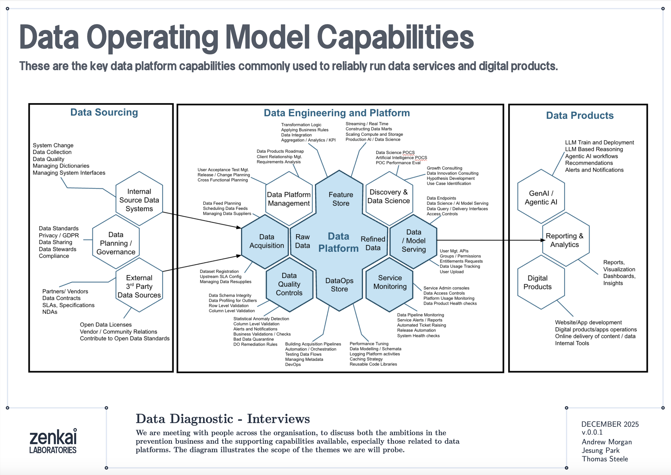
The diagram above shows a reference data operating model organised as a set of capabilities. Data Quality Discovery — the mask-based profiling described in this book — sits as a foundational capability that feeds into Data Quality Monitoring, which in turn feeds into Performance Reporting and Service Assurance. The profiling reports are the raw telemetry; the monitoring architecture is the plumbing that turns telemetry into KPIs; the service assurance layer is where those KPIs drive accountability.

This is not a technology architecture. It is an organisational capability map. The tools described in this book — bytefreq, DataRadar, DuckDB — are implementations. The capabilities they serve are what matter to a CDO or CTO.

Reports as Fact Tables

A standard DQ profile from bytefreq looks like this:

=== Column: postcode ===
Mask                Count   Example
A9 9A               8,412   SW1A 1AA
A99 9A              1,203   M60 1NW
A9A 9A                892   W1D 3QU
9                     312   N/A

In machine-readable mode (JSON output), this becomes a structured record:

{
  "column": "postcode",
  "masks": [
    {"mask": "A9 9A", "count": 8412, "example": "SW1A 1AA"},
    {"mask": "A99 9A", "count": 1203, "example": "M60 1NW"},
    {"mask": "A9A 9A", "count": 892, "example": "W1D 3QU"},
    {"mask": "9", "count": 312, "example": "N/A"}
  ],
  "total": 10819,
  "mask_cardinality": 4
}

Add a feed identifier and a timestamp, and you have a fact record:

{
  "feed": "council-planning-applications",
  "profiled_at": "2025-12-19T08:00:00Z",
  "column": "postcode",
  "masks": [...],
  "total": 10819,
  "mask_cardinality": 4,
  "coverage_top1": 0.777,
  "population_rate": 0.985
}

This is a dimensional fact table. The feed, timestamp, and column are the dimensions. The mask distribution, cardinality, coverage, and population rate are the measures. Store these records consistently and you have a timeseries.

The Directory Pattern

The simplest implementation is a directory of files, partitioned by date and feed:

quality-reports/
  2025-12-18/
    council-planning-applications.dq.ndjson
    council-planning-applications.cp.ndjson
    nhs-patient-demographics.dq.ndjson
    nhs-patient-demographics.cp.ndjson
  2025-12-19/
    council-planning-applications.dq.ndjson
    council-planning-applications.cp.ndjson
    nhs-patient-demographics.dq.ndjson
    nhs-patient-demographics.cp.ndjson

Each file contains the profiling report for one feed on one date. The DQ file contains mask frequency tables per column. The CP file contains character frequency tables. Both are NDJSON — one JSON object per column.

This is the same pool-and-glob pattern described in the DataRadar walkthrough chapter, applied to profiling reports rather than flat enhanced exports. The storage cost is negligible — profiling reports are small (kilobytes, not megabytes) because they contain aggregated frequencies, not individual records.

Querying the Timeseries

DuckDB's file glob turns this directory into a queryable timeseries with no ingestion pipeline:

-- Coverage trend for a specific column across all dates
SELECT
    profiled_at::DATE AS report_date,
    coverage_top1
FROM read_ndjson_auto('quality-reports/*/*.dq.ndjson', filename=true)
WHERE feed = 'council-planning-applications'
  AND column = 'postcode'
ORDER BY report_date;

-- Feeds where mask cardinality increased (new patterns appearing)
SELECT
    feed,
    column,
    profiled_at::DATE AS report_date,
    mask_cardinality
FROM read_ndjson_auto('quality-reports/*/*.dq.ndjson')
WHERE mask_cardinality > 10
ORDER BY feed, column, report_date;

-- Population rate drop detection (mandatory field becoming sparse)
WITH trends AS (
    SELECT
        feed,
        column,
        profiled_at::DATE AS report_date,
        population_rate,
        LAG(population_rate) OVER (
            PARTITION BY feed, column ORDER BY profiled_at
        ) AS prev_rate
    FROM read_ndjson_auto('quality-reports/*/*.dq.ndjson')
)
SELECT * FROM trends
WHERE prev_rate - population_rate > 0.05
ORDER BY report_date DESC;

These are the queries that power a quality dashboard. No database to maintain, no ingestion pipeline to build — just a directory of small JSON files and a query engine that reads them on demand.

Exit Checks and Entrance Checks

The monitoring architecture has two deployment points.

Exit Checks (Producer Side)

An exit check runs after a data pipeline produces its output, before the output is published to consumers. In a CI/CD pipeline, this is a post-build step:

#!/bin/bash
# exit-check.sh — run after data pipeline completes
FEED="council-planning-applications"
DATE=$(date +%Y-%m-%d)
OUTPUT_DIR="quality-reports/${DATE}"
mkdir -p "${OUTPUT_DIR}"

# Profile the output
cat pipeline-output.csv \
  | bytefreq -d ',' -f tabular \
  > "${OUTPUT_DIR}/${FEED}.dq.ndjson"

# Character profile
cat pipeline-output.csv \
  | bytefreq -d ',' -r CP \
  > "${OUTPUT_DIR}/${FEED}.cp.ndjson"

# Check for regressions against previous day
# (custom script that compares today's report with yesterday's)
python3 check-regressions.py \
  --today "${OUTPUT_DIR}/${FEED}.dq.ndjson" \
  --baseline "quality-reports/$(date -d yesterday +%Y-%m-%d)/${FEED}.dq.ndjson"

The exit check produces the quality report and optionally runs regression detection — comparing today's profile against yesterday's to flag significant changes. If the regression check fails (coverage dropped below threshold, new unexpected masks appeared, population rate fell), the pipeline can halt publication and alert the team.

Entrance Checks (Consumer Side)

An entrance check runs when a data feed is received, before it enters the consumer's pipeline:

#!/bin/bash
# entrance-check.sh — run when feed arrives
FEED="council-planning-applications"
DATE=$(date +%Y-%m-%d)
OUTPUT_DIR="quality-reports/${DATE}"
mkdir -p "${OUTPUT_DIR}"

# Profile the received data
cat received-feed.csv \
  | bytefreq -d ',' -E \
  > "${OUTPUT_DIR}/${FEED}.enhanced.ndjson"

cat received-feed.csv \
  | bytefreq -d ',' \
  > "${OUTPUT_DIR}/${FEED}.dq.ndjson"

# Compare against the producer's exit check report
# (if available via shared quality report exchange)
python3 compare-exit-entrance.py \
  --exit "producer-reports/${DATE}/${FEED}.dq.ndjson" \
  --entrance "${OUTPUT_DIR}/${FEED}.dq.ndjson"

When both exit and entrance checks are in place, discrepancies between them reveal problems in transit — encoding changes, truncation, field reordering, or lossy transformations that happened between the producer's output and the consumer's input.

KPIs and the Quality Dashboard

From the timeseries of profiling reports, several KPIs emerge naturally:

Coverage stability — Is the top-1 mask coverage for each column holding steady over time? A sudden drop means a new pattern has appeared in significant volume.

Mask cardinality trend — Is the number of distinct masks per column increasing? A gradual increase may indicate format drift. A sudden spike may indicate a data source change or a pipeline bug.

Population rate — What percentage of each field is populated? Track this daily. A mandatory field that drops from 99.5% to 80% is an early warning of an upstream collection problem.

New mask detection — Did any mask appear today that has never appeared before in this feed? New masks are the single most valuable alert in quality monitoring — they indicate structural change, which may be benign (a new valid format) or problematic (data corruption, source system change, encoding error).

Assertion pass rate — For columns where the rules engine runs (as described in the Assertion Rules Engine chapter), what percentage of values pass their assertions? An IBAN column where is_valid_iban drops from 98% to 85% deserves immediate investigation.

These KPIs are not exotic. They are the data quality equivalent of uptime, latency, and error rate in service monitoring. The difference is that most organisations do not measure them consistently — not because the measurement is hard, but because nobody set up the infrastructure to collect and store the reports. The directory-of-profiles pattern described here makes that infrastructure trivially simple.

Line of Sight: From Impact to Source

The monitoring architecture becomes genuinely powerful when connected to data lineage.

Consider a scenario: a downstream analytics team discovers that 5% of their geospatial analyses are failing because postcodes cannot be geocoded. The entrance check report for the feed shows that 5% of postcode values have the mask aaaa — alphabetic strings like null, none, test. The timeseries shows this started three weeks ago. The feed comes from Council X. Council X's exit check report confirms the same pattern — their collection system started accepting free-text in the postcode field after a software update.

With lineage metadata connecting the feed to its downstream consumers, the impact is quantifiable: 5% of records × N downstream analyses × cost per failed analysis = £Y. This is not a vague "your data is bad" complaint. It is a specific, evidenced, costed impact statement that can be presented to Council X's management.

This is the accountability loop that the introduction described. The timeseries provides the evidence. The lineage provides the traceability. The profiling reports provide the specificity. Together, they enable the conversation: "Your department's data collection change on this date caused this downstream impact costing this amount. Here is the evidence. How shall we fix it?"

Fit for the Journey

The traditional framing of data quality is fit for purpose — can the immediate consumer use the data for their intended task? This is necessary but insufficient.

Data in a modern government or enterprise rarely has one consumer. A dataset collected at a local council may flow through a regional aggregator, a central government data platform, a statistical publication pipeline, a machine learning feature store, and a public API before reaching its final consumers. At each stage, the data is read, interpreted, transformed, and forwarded. At each stage, structural assumptions are made. At each stage, quality issues can be introduced, amplified, or — if the right checks are in place — detected and addressed.

Fit for the journey means the data carries enough structural metadata to be understood and validated at every stage. The flat enhanced format (described in the Flat Enhanced Format chapter) provides this at the record level — each value carries its masks and assertions alongside the raw data. The profiling reports described in this chapter provide it at the feed level — each delivery carries a machine-readable quality certificate that downstream consumers can compare against their expectations.

When a data feed arrives with its profiling report, the consumer does not need to re-profile from scratch (though they may choose to, as an entrance check). They can read the report, compare it against the baseline, and make an informed decision: accept, reject, or accept with caveats. The report is a passport — a document that accompanies the data on its journey and records its structural state at each checkpoint.

Discovery Before Exploration

One final point about where this monitoring architecture sits in the broader data quality landscape.

Mask-based profiling is not a replacement for tools like Great Expectations, dbt tests, Pandas profiling, or Soda. Those tools are excellent at validating known expectations: is this column non-null? Does this value fall within a range? Does this distribution match the historical baseline? They are exploratory and validation tools that assume you already understand the structure of your data well enough to write meaningful tests.

Data Quality Discovery — the mask-based profiling step — comes before exploration. It answers the question that the exploratory tools cannot: what does this data actually look like? You cannot write a Great Expectations test for a column whose structure you have not yet discovered. You cannot explore what you cannot read.

The monitoring architecture described in this chapter adds the time dimension to that discovery. A single profile tells you what the data looks like today. A timeseries of profiles tells you how it is changing. The exit and entrance checks tell you where problems are being introduced. The KPIs tell you whether quality is improving or degrading. And the lineage integration tells you who is affected and what it costs.

These are the building blocks for assuring a data service — not just a file, but the entire flow of data through an organisation. The tools in the following chapters show how to implement each building block. The architecture is how they fit together.

Using DataRadar: A Walkthrough

The previous chapters described the theory: masks, grain levels, population analysis, error codes, treatment functions, and the flat enhanced format. This chapter puts it into practice using DataRadar, the browser-based profiling tool. We will walk through a complete profiling session, from uploading a file to interpreting the output and exporting the results.

Getting Started

Open dataradar.co.uk in any modern browser. There is nothing to install, no account to create, and no data leaves your machine — all processing happens client-side using WebAssembly.

The interface presents a file upload area at the top. You can either click to browse for a file, or drag and drop one onto the page. DataRadar supports four input formats:

• CSV / Tabular — comma, pipe, tab, semicolon, or custom delimited files
• Excel — .xlsx, .xls, .xlsb, and .ods spreadsheets (with sheet selection)
• JSON / NDJSON — newline-delimited JSON (one record per line), or standard JSON arrays
• URLs — paste a URL to a JSON API endpoint and DataRadar will fetch and profile the response directly

For CSV files, the delimiter is auto-detected but can be overridden. For Excel files, you can select which sheet to profile and whether the first row contains headers.

The Report Options

Before running the profiler, three settings control what output you get:

Report Type

• Data Quality (DQ) — the default. Generates mask-based frequency profiles for each column, showing the structural patterns and their counts. This is what you want for the workflow described in this book.
• Character Profiling (CP) — generates byte-level or code-point-level frequency analysis of the file content. This is the forensic mode described in Chapter 5, useful for diagnosing encoding issues, identifying unexpected control characters, or determining the character sets present in the data.

Masking Level

Four grain levels are available:

• High Unicode (HU) — detailed masks with full Unicode character class support. Every character maps individually. This is the default and the most generally useful mode.
• Low Unicode (LU) — compressed masks where consecutive characters of the same class are collapsed. Use this for initial discovery when you want to see structural families rather than exact formats.
• High ASCII (H) — the classic A/a/9 mask at full resolution, treating all non-ASCII bytes as "other." Useful for legacy data or when you specifically want ASCII-only profiling.
• Low ASCII (L) — compressed ASCII masks. The original bytefreq mode, equivalent to the sed one-liner described in Chapter 4.

For most work, start with LU (Low Unicode) to get the broad structural picture, then switch to HU (High Unicode) to examine specific columns in detail.

Output Format

The profiling results can be displayed and exported in several formats:

• Human-readable Text — a formatted report suitable for reading in the browser or pasting into a document.
• JSON — structured output for programmatic consumption.
• Markdown — formatted for inclusion in documentation or GitHub README files.

Running a Profile

With a file loaded and the options set, click Analyze Data. The profiler runs in the browser and results appear below the controls.

The output is organised by column. For each column in the input data, the profiler shows:

• The column name (or column number for headerless files).
• The total count of values profiled.
• A frequency table of masks, sorted by count descending.

For example, profiling a CSV with a phone_number column at High Unicode grain might produce:

=== phone_number (1,000 values) ===

Mask                    Count    %
99999 999999              812   81.2%
+99 9999 999999            95    9.5%
9999 999 9999              42    4.2%
(999) 999-9999             31    3.1%
aaaa                       12    1.2%
99999999999                 4    0.4%
Aaaa aaa Aaaa               2    0.2%
                             2    0.2%

This is the population profile described in Chapter 6. The dominant mask (99999 999999) represents UK mobile numbers. The long tail reveals international formats, US formats, placeholders (aaaa — probably null or none), names in the wrong field (Aaaa aaa Aaaa), and empty strings.

Inspecting the Data

Before running the full profile, DataRadar offers a data preview that shows the first rows of the parsed file. This is worth checking — it confirms that the delimiter was detected correctly, that headers were identified, and that the columns are aligned. If the preview looks wrong (columns misaligned, headers appearing as data rows, or delimiter issues), adjust the format settings and re-check before profiling.

For JSON input, the preview shows the flattened field paths, which is useful for understanding the structure of nested data before profiling it.

The Flat Enhanced Export

The most powerful output mode is the Flat Enhanced JSON export, selected from the Output Format dropdown. This produces the flat enhanced format described in Chapter 9: for every field in every record, the output includes the parallel column families:

{
  "phone_number.raw": "+44 7700 900123",
  "phone_number.HU": "+99 9999 999999",
  "phone_number.LU": "+9 9 9",
  "phone_number.Rules": {
    "string_length": 15,
    "poss_postal_country": null
  },
  "postcode.raw": "SW1A 1AA",
  "postcode.HU": "AA9A 9AA",
  "postcode.LU": "A9A 9A",
  "postcode.Rules": {
    "string_length": 8,
    "is_uk_postcode": true,
    "poss_postal_country": ["UK"]
  }
}

Each record in the input becomes a single JSON line in the output, with every field expanded into its .raw, .HU, .LU, and .Rules sub-columns. This is the file you would load into Pandas, Polars, DuckDB, or any other analytical tool for downstream processing.

Loading Flat Enhanced Output in Python

import pandas as pd

df = pd.read_json('output.ndjson', lines=True)

# Use the raw values
df['postcode.raw']

# Use the mask for quality checks
df['postcode.HU']

# Use the Rules suggestions
df['postcode.Rules'].apply(lambda r: r.get('is_uk_postcode') if r else None)

Loading in DuckDB

SELECT
    "postcode.raw" AS postcode,
    "postcode.HU" AS mask,
    "postcode.Rules"->>'is_uk_postcode' AS is_valid
FROM read_ndjson_auto('output.ndjson');

The real trick comes at scale. In practice, you pool hundreds of small enhanced output files into a single directory — one per source file, one per batch, one per day — and use DuckDB's file glob to query across all of them in one shot:

SELECT
    "postcode.raw" AS postcode,
    "postcode.HU" AS mask,
    "postcode.Rules"->>'is_uk_postcode' AS is_valid,
    filename
FROM read_ndjson_auto('exports/*.ndjson', filename=true)
WHERE "postcode.Rules"->>'is_uk_postcode' = 'false';

This is the pattern that makes mask-based profiling operational. You do not need to merge files, build a database, or maintain an ingestion pipeline. You just drop enhanced exports into a directory and query the lot. DuckDB handles the file glob, schema unification, and columnar scanning — and because the flat enhanced format is regular NDJSON with consistent column names, it all just works. A directory of exports becomes a queryable quality lake with zero infrastructure.

Working With JSON and API Data

One of DataRadar's distinguishing features is its ability to profile JSON data directly, including data fetched from API endpoints. This is particularly useful for open data projects where the data arrives as GeoJSON, REST API responses, or NDJSON feeds.

To profile an API endpoint, paste the URL into the URL field and click fetch. DataRadar will retrieve the response, detect the format, and present it for profiling. If the response is a paginated API response (a single JSON object containing an array), DataRadar detects this and offers to extract and convert the array to NDJSON format automatically.

For example, profiling the USGS earthquake feed:

https://earthquake.usgs.gov/earthquakes/feed/v1.0/summary/all_hour.geojson

DataRadar will detect the nested GeoJSON structure, flatten the properties and geometry objects into dot-notation field paths (properties.time, properties.mag, geometry.coordinates.0), and profile each flattened field. The flat enhanced export then produces output like:

{
  "properties.time.raw": "1766181640870",
  "properties.time.HU": "9999999999999",
  "properties.time.LU": "9",
  "properties.time.Rules": {
    "string_length": 13,
    "is_numeric": true
  }
}

From this output, it is immediately clear that the time field contains 13-digit numeric values — Unix timestamps in milliseconds. A downstream consumer can parse these into datetimes with confidence, knowing that the mask confirms structural consistency across all records.

Multilingual Data

DataRadar handles international data without configuration. When profiling a dataset containing names, addresses, or descriptions in non-Latin scripts, the Unicode-aware masking produces structurally meaningful masks for every script:

• Chinese characters (Lo category) mask to a, so 北京饭店 becomes aaaa
• Arabic text with spaces preserves word boundaries: a a a
• Cyrillic names follow the same uppercase/lowercase distinction as Latin: Aaaaaaa
• Mixed-script fields (Latin + CJK, Arabic + digits) reveal the mixing in the mask

The profiler also reports detected scripts per field, flagging columns that contain mixed scripts — which may indicate encoding issues, data from multiple sources, or legitimate multilingual content.

The Workflow in Practice

A typical DataRadar session follows the two-pass workflow described in Chapter 6:

1. Load the file and check the data preview to confirm correct parsing.
2. Run a Low Unicode (LU) profile to survey the structural landscape. Scan each column's masks to understand the dominant patterns and spot obvious anomalies.
3. Switch to High Unicode (HU) and re-profile to examine specific columns where format precision matters (postcodes, phone numbers, dates, identifiers).
4. Export Flat Enhanced JSON for any data you want to process further — the export preserves raw values, masks, and rule suggestions for every record.
5. Load the export into your analytical tool of choice (Pandas, DuckDB, Excel) and proceed with your analysis, using the mask and Rules columns to guide quality decisions.

The entire process — from opening the browser to having a flat enhanced export loaded in a notebook — typically takes less than five minutes. No installation, no configuration, no data leaving your machine.

For larger datasets — anything beyond roughly 50,000 rows — the browser's memory constraints become the limiting factor. If you hit this ceiling, switch to bytefreq on the command line (see Chapter 13), which handles millions of rows with the same profiling engine and the same output format. DataRadar is for exploration and quick checks; bytefreq is for scale.

Using bytefreq: Installation, Build, and Command-Line Reference

This chapter covers the practical side of bytefreq: how to install it, how to build it from source, and how to use it from the command line. If the previous chapters described the what and why of mask-based profiling, this chapter covers the how.

Prerequisites

bytefreq is written in Rust and built using Cargo, Rust's package manager and build system. If you do not already have Rust installed, the standard installation method is:

curl --proto '=https' --tlsv1.2 -sSf https://sh.rustup.rs | sh

This installs rustc (the compiler), cargo (the build tool), and rustup (the toolchain manager). Follow the on-screen prompts — the defaults are fine for most systems. After installation, restart your terminal or run source $HOME/.cargo/env to make the tools available.

Verify the installation:

rustc --version
cargo --version

Installation

There are two ways to install bytefreq.

From GitHub (recommended)

cargo install --git https://github.com/minkymorgan/bytefreq

This clones the repository, compiles the release binary, and installs it to ~/.cargo/bin/, which should already be on your PATH if Rust is installed correctly.

From a local clone

git clone https://github.com/minkymorgan/bytefreq.git
cd bytefreq
cargo build --release
cargo install --path .

Building from a local clone is useful if you intend to modify the code — for example, to add custom assertion rules as described in the previous chapter.

Verify

bytefreq --version

Input Formats

bytefreq supports four input formats:

Tabular (-f tabular, the default) — delimited text where the first line is a header row and subsequent lines are data records. The delimiter defaults to pipe (|) but can be set to any character using the -d flag. Tabular data is read from standard input (stdin).

JSON (-f json) — newline-delimited JSON (NDJSON), where each line is a complete JSON object. bytefreq flattens nested structures using dot-notation paths (e.g., customer.address.postcode), handling arrays and nested objects to a configurable depth. JSON data is read from standard input.

Excel (-f excel --excel-path file.xlsx) — native Excel file support for .xlsx, .xls, .xlsb, and .ods formats. Requires building with the excel feature flag (cargo install --git https://github.com/minkymorgan/bytefreq --features excel). By default, bytefreq reads the first sheet; use --excel-sheet to select a specific sheet by index (0-based).

Parquet (-f parquet --parquet-path file.parquet) — native Apache Parquet file support. Requires building with the parquet feature flag (cargo install --git https://github.com/minkymorgan/bytefreq --features parquet). Parquet files are converted internally to JSON lines, so all JSON features — dot-notation nested paths, array index handling (-a), path depth limiting (-p), and enhanced output — work with Parquet data. Nested structs produce dot-notation paths (user.address.city), and list columns produce indexed array paths (scores[0], scores[1]). Timestamps are automatically converted to ISO 8601 strings, and all standard Arrow data types are supported.

To install with all optional format support:

cargo install --git https://github.com/minkymorgan/bytefreq --features parquet,excel

A note on CSV: bytefreq defaults to pipe-delimited input rather than comma-delimited, because pipe characters appear far less frequently in real-world data values and thus produce fewer parsing ambiguities. If your data is comma-delimited, pass -d ','. For complex CSV files with quoted fields, escaped delimiters, or embedded newlines, bytefreq uses a proper CSV parser that handles quoted fields and escape sequences correctly.

Command-Line Reference

bytefreq [OPTIONS]

OPTIONS:
  -g, --grain <GRAIN>          Masking grain level [default: LU]
                                 H  - High grain ASCII (A/a/9)
                                 L  - Low grain ASCII (compressed)
                                 U  - High grain Unicode (HU)
                                 LU - Low grain Unicode (compressed)

  -d, --delimiter <DELIM>      Field delimiter [default: |]

  -f, --format <FORMAT>        Input format [default: tabular]
                                 tabular - Delimited text with header
                                 json    - Newline-delimited JSON
                                 excel   - Excel file (requires --excel-path)
                                 parquet - Parquet file (requires --parquet-path)

      --excel-path <PATH>      Path to Excel file (with -f excel)
      --excel-sheet <INDEX>    Sheet index, 0-based [default: 0]
      --parquet-path <PATH>    Path to Parquet file (with -f parquet)

  -r, --report <REPORT>        Report type [default: DQ]
                                 DQ - Data Quality (mask frequencies)
                                 CP - Character Profiling (byte/codepoint frequencies)

  -p, --pathdepth <DEPTH>      JSON nesting depth [default: 9]

  -a, --remove-array-numbers   Collapse array indices in JSON paths

  -e, --enhanced-output        Output flat enhanced JSON (nested format)

  -E, --flat-enhanced           Output flat enhanced JSON (flattened format)

  -h, --help                   Print help
  -V, --version                Print version

Basic Profiling

The most common use case is profiling a delimited file at the default grain level (Low Unicode):

cat data.csv | bytefreq -d ','

The output is a human-readable frequency report, organised by column. For each column, bytefreq lists the unique masks found, their occurrence counts, and a randomly sampled example value for each mask (selected using reservoir sampling to ensure a truly random representative):

=== Column: postcode ===
Mask                Count   Example
A9 9A               8,412   SW1A 1AA
A99 9A              1,203   M60 1NW
A9A 9A                892   W1D 3QU
AA9 9A                567   EC2R 8AH
9                     312   N/A
                       44

The example column is particularly useful during exploratory profiling — it lets you see an actual value behind each mask without having to go back to the raw data.

Grain Levels in Practice

Low Unicode (LU) — the default

cat data.csv | bytefreq -d ',' -g LU

Consecutive characters of the same Unicode class are collapsed. Good for initial discovery: how many structural families exist in each column?

High Unicode (HU) — exact formats

cat data.csv | bytefreq -d ',' -g HU

Every character maps individually. Good for precision work: what exact postcode formats are present? What date formats are in use?

High ASCII (H) and Low ASCII (L) — legacy modes

cat data.csv | bytefreq -d ',' -g H
cat data.csv | bytefreq -d ',' -g L

The original A/a/9 masks without Unicode awareness. All non-ASCII characters are left unmapped. Useful when profiling data known to be ASCII-only, or when comparing results against the legacy awk-based bytefreq.

Character Profiling

The -r CP flag switches from mask-based profiling to character-level frequency analysis:

cat data.csv | bytefreq -d ',' -r CP

This reports the frequency of every Unicode code point found in the file, alongside the character itself and its Unicode name. The output is sorted by frequency and grouped by Unicode General Category (Letter, Number, Punctuation, Symbol, Separator, Other).

Character profiling is the forensic tool. Use it when you need to:

• Determine the encoding of an unknown file — UTF-8, Latin-1, Windows-1252, and mixed encodings each produce characteristic byte patterns.
• Find invisible characters — zero-width spaces, byte order marks, soft hyphens, and other non-printing characters that cause subtle parsing failures.
• Detect control characters — tabs, carriage returns, null bytes, and other control characters in fields that should contain only printable text.
• Understand the script composition — what proportion of the text is Latin, Cyrillic, CJK, Arabic, or other scripts?

JSON Profiling

For JSON data, use -f json:

cat data.ndjson | bytefreq -f json

bytefreq expects newline-delimited JSON — one complete JSON object per line. It flattens nested structures into dot-notation paths:

{"customer": {"address": {"postcode": "SW1A 1AA"}}}

becomes a column named customer.address.postcode with value SW1A 1AA.

Controlling nesting depth

For deeply nested JSON, the -p flag controls how many levels of nesting bytefreq will traverse. Consider this input:

{"org": {"dept": {"team": {"lead": {"name": "Alice"}}}}}

With the default depth (-p 9), this produces a column named org.dept.team.lead.name. Limiting the depth changes what bytefreq sees:

# Full depth — profiles org.dept.team.lead.name
cat data.ndjson | bytefreq -f json

# Depth 3 — profiles org.dept.team (stops here, treats remaining nesting as a value)
cat data.ndjson | bytefreq -f json -p 3

# Depth 1 — profiles org (the entire nested object as a single JSON string)
cat data.ndjson | bytefreq -f json -p 1

Limiting depth is useful for very complex JSON structures where the full path depth produces an unmanageable number of columns. Start shallow and increase depth as needed.

Collapsing array indices

JSON arrays produce indexed paths by default. Given this input:

{"items": [{"name": "Widget"}, {"name": "Gadget"}, {"name": "Doohickey"}]}

bytefreq generates separate columns: items.0.name, items.1.name, items.2.name. The -a flag collapses the array index, treating all array elements as the same column:

# Without -a: items.0.name, items.1.name, items.2.name (3 separate columns)
cat data.ndjson | bytefreq -f json

# With -a: items.name (1 column, all array elements pooled together)
cat data.ndjson | bytefreq -f json -a true

This produces items.name instead of separate columns per array position, which is usually what you want for profiling the structural patterns within array elements. The collapsed column's mask frequency table then reflects the patterns across all array elements, not just those at a specific index.

Enhanced Output

The -e and -E flags switch bytefreq from profiling mode to enhanced output mode. Instead of producing a frequency report, the tool processes every record and outputs the flat enhanced format described in Chapter 9.

Nested enhanced (-e)

cat data.csv | bytefreq -d ',' -e

Produces one JSON object per input row, with each field expanded into a nested structure:

{
  "postcode": {
    "raw": "SW1A 1AA",
    "HU": "AA9A 9AA",
    "LU": "A9A 9A",
    "Rules": {
      "string_length": 8,
      "is_uk_postcode": true,
      "poss_postal_country": ["UK"]
    }
  }
}

Flat enhanced (-E)

cat data.csv | bytefreq -d ',' -E

Produces the same information but flattened to dot-notation keys — one level deep, no nesting:

{
  "postcode.raw": "SW1A 1AA",
  "postcode.HU": "AA9A 9AA",
  "postcode.LU": "A9A 9A",
  "postcode.Rules.string_length": 8,
  "postcode.Rules.is_uk_postcode": true,
  "postcode.Rules.poss_postal_country": ["UK"]
}

The flat format is easier to load into columnar tools (Pandas, DuckDB, Parquet) because every key maps directly to a column name without requiring nested JSON parsing.

Pipeline Recipes

bytefreq is designed for Unix pipelines. Here are some common patterns:

Profile the first 10,000 rows of a large file

head -10001 data.csv | bytefreq -d ','

(10,001 to include the header row.)

Profile compressed data

zcat data.csv.gz | bytefreq -d ','

Profile a remote API response

curl -s 'https://api.example.com/data' | bytefreq -f json

Generate flat enhanced output and load into DuckDB

cat data.csv | bytefreq -d ',' -E > enhanced.ndjson
duckdb -c "SELECT * FROM read_ndjson_auto('enhanced.ndjson') LIMIT 10;"

Profile only specific columns (using pre-processing)

cat data.csv | cut -d',' -f1,3,5 | bytefreq -d ','

Compare two files structurally

diff <(cat file1.csv | bytefreq -d ',') <(cat file2.csv | bytefreq -d ',')

This shows which columns have gained or lost structural patterns between two versions of the same dataset — useful for detecting format drift over time.

Profile an Excel file (native)

bytefreq -f excel --excel-path data.xlsx

To profile a specific sheet (0-based index):

bytefreq -f excel --excel-path data.xlsx --excel-sheet 2

(Requires building with --features excel. Alternatively, DataRadar handles Excel files natively in the browser.)

Profile a Parquet file

bytefreq -f parquet --parquet-path data.parquet

Nested structs produce dot-notation paths and list columns produce indexed array paths, just like JSON. Use -a to collapse array indices:

bytefreq -f parquet --parquet-path data.parquet -a

Generate flat enhanced output from Parquet:

bytefreq -f parquet --parquet-path data.parquet -E > enhanced.ndjson

(Requires building with --features parquet.)

Understanding the Output

The standard DQ report output follows a consistent format:

=== Column: field_name ===
Mask                Count   Example
aaaa.aaaa@aaaa.aaa  45,231  john.smith@email.com
aaaa@aaaa.aaa        8,102  jane@company.org
Aaaa Aaaaa             312  John Smith
99999                   45  12345
                        12
--------END OF REPORT--------

Each section corresponds to one column in the input. Masks are sorted by descending frequency, so the most common patterns appear first. The example value is a true random sample selected using reservoir sampling — not the first occurrence, but a statistically representative one.

The --------END OF REPORT-------- marker signals the end of the output, which is useful when piping to downstream tools.

Performance

bytefreq uses Rayon for multi-threaded processing, so it will utilise all available CPU cores when generating enhanced output. For standard DQ profiling, the bottleneck is typically I/O rather than computation — the mask function is simple enough that CPU time is negligible compared to the time spent reading input.

On a modern machine, expect throughput of several hundred thousand rows per second for tabular data, depending on the number of columns and the average field length. For most datasets under a few million rows, profiling completes in seconds.

The Assertion Rules Engine: Inside bytefreq

The preceding chapters described the DQOR framework conceptually — masks, population analysis, error codes, treatment functions, and the flat enhanced format. This chapter opens the bonnet. We will walk through the actual Rust code that implements assertion rules in bytefreq, show how the rules engine works, and explain how to add a new rule. If you are not a Rust programmer, do not worry — the patterns are straightforward and the logic reads more like pseudocode than systems programming. The important thing is the design patterns, not the language syntax.

Architecture

The rules engine in bytefreq is deliberately simple. It consists of two files in the src/rules/ directory:

• assertions.rs — a library of assertion functions, each of which examines a (field_name, raw, HU, LU) tuple and returns zero or more assertions about the value.
• enhancer.rs — a thin orchestration layer that calls execute_assertions and returns the results.

When bytefreq runs in enhanced mode (-e or -E), every value in the input is processed through a pipeline:

1. The raw value is read from the input (CSV column, JSON field, etc.).
2. The HU (high-grain Unicode) and LU (low-grain Unicode) masks are generated.
3. The triple (raw, HU, LU) is passed to the rules engine along with the field name.
4. The rules engine runs all applicable assertions and returns a JSON object.
5. The output is written in the flat enhanced format: { "raw": ..., "HU": ..., "LU": ..., "Rules": ... }.

The processing is parallelised across columns using Rayon, so on a multi-core machine the assertion checks run concurrently for each field in a row:

#![allow(unused)]
fn main() {
fn process_tabular_line_as_json(
    processed_fields: &Vec<(String, String)>
) -> serde_json::Value {
    let json_line: HashMap<String, serde_json::Value> = processed_fields
        .par_iter()
        .map(|(column_name, value)| {
            let hu_masked_value = mask_value(value, "HU", column_name);
            let lu_masked_value = mask_value(value, "LU", column_name);

            let data = json!({
                "raw": value,
                "LU": lu_masked_value,
                "HU": hu_masked_value
            });

            let assertions = process_data(&column_name, &data);

            let enhanced_value = json!({
                "raw": value,
                "HU": hu_masked_value,
                "LU": lu_masked_value,
                "Rules": assertions
            });

            (column_name.clone(), enhanced_value)
        })
        .collect();

    serde_json::Value::Object(json_line.into_iter().collect())
}
}

The key thing to notice is that the assertion rules receive the mask as well as the raw value. This is the design pattern that makes the engine efficient: the mask acts as a fast structural filter, allowing rules to skip values that are structurally irrelevant without parsing or interpreting them.

The Enhancer

The enhancer (src/rules/enhancer.rs) is intentionally minimal:

#![allow(unused)]
fn main() {
use crate::rules::assertions::execute_assertions;

pub fn process_data(
    field_name: &str,
    data: &serde_json::Value
) -> Option<serde_json::Value> {
    let lu = data["LU"].as_str().unwrap_or("");
    let hu = data["HU"].as_str().unwrap_or("");
    let raw = data["raw"].as_str().unwrap_or("");

    let assertions = execute_assertions(field_name, raw, lu, hu);

    if assertions.as_object().unwrap().is_empty() {
        None
    } else {
        Some(assertions)
    }
}
}

It extracts the triple from the JSON structure, calls execute_assertions, and returns None if no rules matched (keeping the output sparse — fields with no applicable rules produce no Rules column, which saves space in the flat enhanced output).

The Assertions Library

The core of the engine is execute_assertions in src/rules/assertions.rs. This function takes the field name, raw value, LU mask, and HU mask, and builds up a JSON object of assertions:

#![allow(unused)]
fn main() {
pub fn execute_assertions(
    field_name: &str,
    raw: &str,
    lu: &str,
    hu: &str
) -> serde_json::Value {
    let mut assertions: serde_json::Map<String, serde_json::Value> =
        serde_json::Map::new();

    // Always compute string length
    assertions.insert(
        "string_length".to_string(),
        json!(string_length(raw))
    );

    // Postal code country detection — only if field name contains "post"
    if field_name.to_lowercase().contains("post") {
        let possible_countries = get_possible_countries(
            field_name, raw, hu, lu
        );
        if !possible_countries.is_empty() {
            assertions.insert(
                "poss_postal_country".to_string(),
                json!(possible_countries)
            );
        }
    }

    // Country name standardisation
    if field_name.to_lowercase().contains("country")
        && !lu.chars().any(|c| c.is_numeric())
    {
        if let Some((iso3, region_code)) = country_name_to_iso3(raw)
            .map(|iso3| (iso3.clone(), format!("{}-{}", iso3, raw)))
            .or_else(|| handle_country_name_variations(raw))
        {
            assertions.insert("std_country_iso3".to_string(), json!(iso3));
            assertions.insert("std_region_code".to_string(), json!(region_code));
        }
    }

    // Numeric detection
    if lu == "9" || lu == "9.9" {
        assertions.insert(
            "is_numeric".to_string(),
            json!(is_numeric(raw))
        );
    }

    // UK postcode validation
    if lu == "A9 9A" || hu == "A9A 9A" {
        assertions.insert(
            "is_uk_postcode".to_string(),
            json!(is_uk_postcode(raw))
        );
    }

    // Date parsing
    if lu == "9_9_9" {
        assertions.insert(
            "std_date".to_string(),
            json!(parse_date(raw))
        );
    }

    // Date of birth sensibility check
    if hu == "99_99_9999" && field_name.to_lowercase().contains("dob") {
        assertions.insert(
            "is_sensible_dob".to_string(),
            json!(is_sensible_dob(raw))
        );
    }

    serde_json::Value::Object(assertions)
}
}

There are several design patterns worth noting here.

Pattern 1: Mask-Gated Rules

Most rules are gated by the LU or HU mask. The UK postcode check only fires when lu == "A9 9A" — meaning the value structurally looks like a postcode (letters, digits, space, digits, letters). The date parser only fires when lu == "9_9_9" — meaning the value has three groups of digits separated by a non-digit character. The numeric check only fires when lu == "9" or lu == "9.9".

This is efficient. Rather than running every assertion against every value (which would be wasteful for a million-row file with dozens of columns), the mask pre-filters. A name column with mask Aaaa Aaaaa will skip the postcode check, the numeric check, and the date parser entirely. Only rules whose structural precondition matches the mask will execute.

This is the same principle introduced in Chapter 7 (Masks as Error Codes), but applied in reverse: instead of using masks to detect problems, we use them to select which enhancement rules are applicable.

Pattern 2: Field-Name-Aware Rules

Some rules use the field name as additional context. The postal country detection only runs when the field name contains "post". The country name standardisation only runs when the field name contains "country". The date-of-birth sensibility check only runs when the field name contains "dob".

This is a pragmatic heuristic. A value of SW1A 1AA in a field called postcode should be checked as a UK postcode. The same value in a field called reference_code probably should not. The field name provides domain context that the mask alone cannot.

The heuristic is deliberately loose — contains("post") will match postcode, postal_code, home_postcode, post_code, and even post_office_box. This is intentional: it is better to over-match and produce an assertion that the consumer can ignore, than to under-match and miss a useful suggestion.

Pattern 3: Standardisation Suggestions

Several rules do not just detect a property but suggest a standardised form. The country name rule maps free-text country names to ISO 3166-1 alpha-3 codes:

#![allow(unused)]
fn main() {
fn country_name_to_iso3(value: &str) -> Option<String> {
    let name_to_iso3 = country(|c| (
        c.name.to_lowercase(),
        c.iso3
    ));
    name_to_iso3
        .get(&value.to_lowercase())
        .map(|s| s.to_string())
}
}

The function uses the geonamescache crate to look up country names against a known dictionary, returning the ISO3 code if a match is found. It also handles common variations that the standard dictionary misses — "England", "Scotland", "Wales", and "Northern Ireland" are mapped to their ISO codes with region suffixes:

#![allow(unused)]
fn main() {
fn handle_country_name_variations(country_name: &str) -> Option<(String, String)> {
    match country_name.to_lowercase().as_str() {
        "england"          => Some(("GBR".to_string(), "GB-ENG".to_string())),
        "scotland"         => Some(("GBR".to_string(), "GB-SCT".to_string())),
        "northern ireland" => Some(("GBR".to_string(), "GB-NIR".to_string())),
        "wales" | "cymru"  => Some(("GBR".to_string(), "GB-WLS".to_string())),
        _ => None,
    }
}
}

The output in the Rules column would look like:

{
  "std_country_iso3": "GBR",
  "std_region_code": "GBR-England"
}

This is a suggestion, not a correction. The raw value "England" is preserved in the .raw column. The consumer can choose to use the ISO3 code, or keep the original, or apply their own mapping. The engine surfaces the assertion; the consumer decides what to do with it.

Pattern 4: Postal Code Country Detection

The get_possible_countries function is a particularly good example of mask-driven inference. It uses the HU mask of a postal code to determine which countries could have produced that format:

#![allow(unused)]
fn main() {
fn get_possible_countries(
    _column_name: &str, raw: &str, hu: &str, lu: &str
) -> Vec<String> {
    let mut possible_countries: Vec<String> = Vec::new();

    match hu {
        "9999" => {
            possible_countries.extend(vec![
                "AT", "BE", "BG", "CH", "CY", "CZ", "DK", "EE",
                "FI", "GR", "HU", "IE", "LT", "LU", "LV", "MT",
                "NL", "NO", "PL", "PT", "RO", "SE", "SI", "SK"
            ].into_iter().map(|s| s.to_string()));
        }
        "99999" => {
            possible_countries.extend(vec![
                "DE", "ES", "FR", "HR", "IT"
            ].into_iter().map(|s| s.to_string()));
        }
        "999-99" => {
            possible_countries.push("SE".to_string());
        }
        "AAA-9999" => {
            possible_countries.push("IE".to_string());
        }
        _ => {}
    }

    // Refine using value-level checks
    if lu == "9-9999" && raw.starts_with("1") {
        possible_countries.retain(|c| c == "DE");
    }

    // UK postal code patterns
    let uk_patterns = vec!["A9 9A", "A9A 9A", "A9A"];
    if uk_patterns.contains(&lu) {
        possible_countries.push("UK".to_string());
    }

    possible_countries
}
}

Notice the two-level logic. First, the HU mask narrows the field to a set of possible countries (a 4-digit postal code could be Austrian, Belgian, Swiss, etc.). Then, value-level checks refine the set further (a 4-digit code starting with 0 is likely Dutch; a 5-digit code starting with 9 is likely French). The result is a list of possible countries, not a definitive answer — again, a suggestion that the consumer can use to inform their own logic.

Implementing a New Rule

Adding a new assertion rule to bytefreq involves three steps.

Step 1: Write the Detection Function

Create a function in assertions.rs that takes a raw value (and optionally the masks or field name) and returns the assertion result. For example, a rule to detect email addresses:

#![allow(unused)]
fn main() {
pub fn is_email(value: &str) -> bool {
    let re = Regex::new(
        r"^[a-zA-Z0-9._%+-]+@[a-zA-Z0-9.-]+\.[a-zA-Z]{2,}$"
    ).unwrap();
    re.is_match(value)
}

pub fn extract_email_domain(value: &str) -> Option<String> {
    value.split('@').nth(1).map(|s| s.to_lowercase())
}
}

Step 2: Wire It Into execute_assertions

Add a conditional block in the execute_assertions function, gated by the appropriate mask pattern:

#![allow(unused)]
fn main() {
// Email detection — LU mask "a@a.a" covers most email patterns
if lu.contains("@") && lu.contains(".") {
    assertions.insert(
        "is_email".to_string(),
        json!(is_email(raw))
    );
    if let Some(domain) = extract_email_domain(raw) {
        assertions.insert(
            "email_domain".to_string(),
            json!(domain)
        );
    }
}
}

The mask gate here is simple: if the LU mask contains both @ and ., the value might be an email address (since those punctuation characters are preserved in the mask). The is_email function then performs the definitive check, and extract_email_domain provides a standardised extraction.

Step 3: Build and Test

cargo build
echo 'name,email,postcode
John Smith,john@example.com,SW1A 1AA
Jane Doe,jane.doe@company.co.uk,EC2R 8AH' | cargo run -- -E

The output for the email column would include:

{
  "email": {
    "raw": "john@example.com",
    "HU": "aaaa@aaaaaaa.aaa",
    "LU": "a@a.a",
    "Rules": {
      "string_length": 16,
      "is_email": true,
      "email_domain": "example.com"
    }
  }
}

Design Guidelines for New Rules

When writing a new assertion rule, several principles from the existing codebase are worth following:

Gate by mask first. The mask check should be the outer conditional, because it is essentially free (a string comparison) and filters out the majority of values that cannot possibly match. Only values that pass the mask gate should incur the cost of the full assertion logic (regex matching, parsing, dictionary lookup, etc.).

Use the field name as a hint, not a requirement. Field-name matching (field_name.contains("post")) is useful for disambiguation but should not be the only gate. Some datasets have opaque field names (col_7, field_12), and the rule should still fire for structurally matching values even when the field name provides no context.

Return suggestions, not corrections. The assertion should describe what the value is or what it could be, not what it should be changed to. The consumer decides whether to act on the suggestion. This keeps the rules engine non-destructive and maintains the DQOR principle of preserving the raw value.

Cache expensive lookups. The country name lookup uses a RwLock<HashMap> cache to avoid repeated dictionary scans. Any rule that performs an expensive operation (network call, large dictionary lookup, complex regex compilation) should cache results for values it has seen before. The lazy_static pattern used for the country cache is a good template:

#![allow(unused)]
fn main() {
lazy_static! {
    pub static ref COUNTRY_NAME_TO_ISO3_CACHE:
        RwLock<HashMap<String, Option<String>>> =
            RwLock::new(HashMap::new());
}
}

Keep rules independent. Each rule should be self-contained. Rules should not depend on the output of other rules, and the order in which they execute should not matter. This allows the engine to run rules in parallel (which it does via Rayon) and makes it safe to add, remove, or modify rules without side effects.

The Rules as a Living Library

The assertion rules in bytefreq are not a closed set. They are a starting point — a library of common patterns that cover postal codes, country names, dates, numeric values, and basic structural properties. As the tool encounters new types of data, new rules are added.

This is the same continuous improvement loop described in Chapter 8 (treatment functions): profile the data, discover new patterns, write rules to detect and characterise them, and add the rules to the library. Over time, the library grows to reflect the kinds of data that bytefreq's users actually encounter, making the flat enhanced output increasingly useful with each release.

The rules are also an invitation. Because the engine is open source and the pattern for adding a new rule is straightforward — write a function, gate it by mask, wire it into execute_assertions — users with domain-specific knowledge can contribute rules for their own data types. The mask-gated architecture means domain-specific rules coexist with the general-purpose ones without interference, and the flat enhanced format ensures that all assertions — general and domain-specific — are delivered to consumers in a consistent structure.

To make this concrete, here are sketches for three domain-specific rules that follow the same patterns described above.

Example: NHS Number Validation (Healthcare)

An NHS number is a 10-digit identifier with a modulus 11 check digit. The mask gate is simple: hu == "9999999999" (exactly 10 digits). The validation function computes the weighted sum and checks the remainder:

#![allow(unused)]
fn main() {
// Gate: hu == "9999999999"
pub fn is_nhs_number(value: &str) -> bool {
    let digits: Vec<u32> = value.chars().filter_map(|c| c.to_digit(10)).collect();
    if digits.len() != 10 { return false; }
    let weighted_sum: u32 = digits[..9].iter()
        .enumerate()
        .map(|(i, &d)| d * (10 - i as u32))
        .sum();
    let remainder = weighted_sum % 11;
    let check = if remainder == 0 { 0 } else { 11 - remainder };
    check != 10 && check == digits[9]
}
}

The mask gate ensures this function never fires on phone numbers, postcodes, or other 10-digit values in columns that are not plausibly NHS numbers. A field-name hint (field_name.contains("nhs") or field_name.contains("patient")) could narrow it further.

Example: IBAN Detection (Financial Services)

An IBAN starts with a two-letter country code, followed by two check digits, followed by a country-specific Basic Bank Account Number (BBAN). The HU mask for a GB IBAN looks like AA99AAAA99999999999999 — 22 characters, letters then digits. The mask gate targets this family of patterns:

#![allow(unused)]
fn main() {
// Gate: hu starts with "AA99" and length matches known IBAN lengths
pub fn is_valid_iban(value: &str) -> bool {
    let clean: String = value.chars().filter(|c| !c.is_whitespace()).collect();
    if clean.len() < 15 || clean.len() > 34 { return false; }
    // Move first 4 chars to end, convert letters to digits (A=10..Z=35)
    let rearranged = format!("{}{}", &clean[4..], &clean[..4]);
    let numeric: String = rearranged.chars().map(|c| {
        if c.is_alphabetic() {
            format!("{}", c.to_ascii_uppercase() as u32 - 55)
        } else {
            c.to_string()
        }
    }).collect();
    // Modulus 97 check
    numeric.chars().fold(0u64, |acc, c| {
        (acc * 10 + c.to_digit(10).unwrap() as u64) % 97
    }) == 1
}
}

The output might include both validation and decomposition:

{
  "is_iban": true,
  "iban_country": "GB",
  "iban_bban": "NWBK60161331926819"
}

Example: Email Address Detection

The email rule shown in the "Implementing a New Rule" section above is another example of the pattern. The mask gate (lu.contains("@") && lu.contains(".")) is structural, the validation is semantic, and the extraction (email_domain) provides a useful standardisation suggestion. Together, these three examples — healthcare, financial services, and general-purpose — illustrate how the same mask-gate-then-validate pattern extends to any domain.

Conclusion

Mask-based profiling is not a silver bullet. It will not catch semantic errors — a phone number that is structurally valid but belongs to the wrong person, a date that is correctly formatted but factually wrong, a numeric value that parses fine but represents a measurement in the wrong units. It will not replace domain expertise, business validation rules, or statistical anomaly detection. Those techniques have their place, and they should continue to be used where they are appropriate.

Mask-based profiling is complementary to tools like Great Expectations, dbt tests, and Soda — not a replacement for them. Those tools excel at validating known expectations: is this column non-null? Does this value fall within a range? Does this foreign key relationship hold? Mask-based profiling excels at discovering what you did not know to expect. Use DQOR to explore and characterise the data first, then encode what you learn as expectations in whatever validation framework your pipeline already uses. The masks tell you what to test for; the validation tools enforce the tests.

What mask-based profiling does, and does exceptionally well, is provide a fast, assumption-free structural census of any dataset at the point of consumption. It answers the question "what does this data actually look like?" before you invest time and resources in trying to use it. It generates quality metadata — masks, population profiles, error codes — as a side effect of profiling, at no additional cost. And it does so deterministically, reproducibly, and at any scale from a single CSV in a browser to billions of records on a Spark cluster.

The Data Quality on Read architecture that surrounds the technique — raw data preservation, deferred quality processing, the flat enhanced format, treatment functions keyed by mask — is designed for the reality of modern data work, where the data you need to use was created by someone else, documented imperfectly, and delivered with whatever level of quality the source system happened to produce. You cannot control the source. What you can control is how quickly and cheaply you understand what you have received, and how systematically you address the issues you find.

The tools are open source. The technique is simple enough to prototype in a single line of sed and powerful enough to run in production at enterprise scale. The hardest part, as with most things in data engineering, is not the technology but the discipline: profiling consistently, documenting what you find, building the quality loop, and maintaining it over time.

If there is a single lesson from nearly two decades of applying this technique across financial services, telecoms, government, and open data projects, it is this: the data is never as clean as the specification says it is, the specification is never as accurate as the author believes it is, and the cost of discovering these facts late is always higher than the cost of discovering them early.

Profile early. Profile often. Let the masks speak for themselves.

If you are ready to try the technique, the Getting Started appendix has everything you need to run your first profile in under a minute.

Glossary

This glossary defines the key technical terms used throughout this book. In translated editions, these terms are kept in English to maintain consistency with the tools and code examples. The definitions below serve as the reference for all translations.

allow list — A list of masks that are considered acceptable for a given column. Values whose masks do not appear in the allow list are flagged as anomalies. Compare with exclusion list.

assertion — A property or suggestion automatically inferred by the rules engine about a data value. For example, is_uk_postcode: true or std_country_iso3: "GBR". Assertions are advisory — consumers choose whether to act on them.

bytefreq — An open-source command-line data profiling tool, written in Rust, that implements mask-based profiling and the flat enhanced output format. Originally written in awk in 2007. Short for byte frequencies.

character class — A category of character defined by the Unicode General Category standard: uppercase letter (Lu), lowercase letter (Ll), digit (Nd), punctuation, symbol, separator, and so on. Mask-based profiling translates each character to a symbol representing its class.

character profiling (CP) — A report mode that analyses the frequency of individual byte values or Unicode code points in a file. Used for encoding detection, invisible character discovery, and script composition analysis. Compare with data quality profiling.

coverage — The percentage of values in a column that match the top N masks. High coverage (>95%) indicates a structurally uniform column; low coverage indicates structural diversity.

DataRadar — A browser-based data quality profiling tool that runs entirely client-side using WebAssembly. Implements the same profiling engine as bytefreq. Available at dataradar.co.uk.

data quality on read (DQOR) — An architecture principle where data quality profiling, validation, and remediation are deferred until the moment of consumption, rather than applied at ingest time. A parallel to schema on read.

cliff point — The point in a sorted mask frequency table where the percentage-of-previous-mask drops sharply, separating expected patterns from rare exceptions. Used for management by exception: masks above the cliff are normal operations; masks below it form a review queue for potential new assertion rules or treatment functions.

data quality profiling (DQ) — The default report mode in bytefreq and DataRadar. Generates mask frequency tables for each column, showing structural patterns and their occurrence counts.

exclusion list — A list of masks that are known to be problematic for a given column. Values whose masks match the exclusion list are flagged as errors. Compare with allow list.

flat enhanced format — A flattened key-value pair schema, sourced from nested data. Each field in the original data is expanded into a family of dot-notated keys: .raw (original value), .HU (high-grain mask), .LU (low-grain mask), and .Rules (assertions and suggestions). The floating schema handles ragged rows gracefully, annotations are easily added, and the namespace dot notation provides provenance and scoping.

grain — The resolution level of a mask. High grain maps every character individually, preserving exact lengths. Low grain collapses consecutive characters of the same class into a single symbol, reducing cardinality for structural discovery.

HU (High Unicode) — High-grain masking with Unicode character class support. Every character maps individually using its Unicode General Category. The most detailed masking level.

LU (Low Unicode) — Low-grain masking with Unicode support. Consecutive characters of the same class are collapsed. The default masking level in bytefreq, and the recommended starting point for exploratory profiling.

mask — A structural fingerprint of a data value, produced by translating each character to a symbol representing its character class. Uppercase letters become A, lowercase become a, digits become 9, and punctuation is kept as-is. For example, John Smith produces the mask Aaaa Aaaaa.

mask cardinality — The number of distinct masks found in a column. Low cardinality (1–3 masks) indicates a well-structured column; high cardinality may indicate structural diversity or data quality issues.

population check — A test that determines whether each field in a record is populated or empty. When aggregated, it produces a per-field population percentage showing the proportion of non-null values.

population profile — A frequency table of masks for a column, sorted by count. Shows the dominant structural patterns and the long tail of rare masks.

Rayon — A Rust library for data parallelism that enables multi-threaded processing with minimal code changes. bytefreq uses Rayon to parallelise mask generation and assertion rule evaluation across columns, utilising all available CPU cores automatically.

provenance — The ability to trace a derived or treated value back to the original raw value it was computed from. The flat enhanced format preserves provenance by keeping the .raw column immutable alongside all derived columns.

.raw — The column in the flat enhanced format that contains the original, untouched value exactly as received from the source. Never modified, never overwritten.

reservoir sampling — A statistical technique used by bytefreq to select a truly random example value for each mask in a profiling report, without requiring a second pass over the data.

.Rules — The column in the flat enhanced format that contains automatically inferred assertions and suggested treatments for a value. Rules are advisory, not prescriptive — multiple competing suggestions can coexist.

schema on read — A data architecture principle where structural interpretation is deferred until the point of consumption, rather than enforced at ingest time. The foundation of modern data lake architectures, and the conceptual predecessor of data quality on read.

script detection — Automatic identification of the dominant Unicode scripts present in each column (e.g., Latin, Cyrillic, Arabic, CJK). Used to flag encoding issues and inform downstream processing.

treatment function — A remediation action mapped to a specific (column, mask) combination. For example, applying title-case normalisation to values with the mask AAAA AAAAA, or replacing placeholder values (mask A/A) with nulls. Treatment functions are non-destructive — the original value is always preserved.

WebAssembly (WASM) — A binary instruction format that allows code written in languages like Rust to run in web browsers at near-native speed. DataRadar uses WASM to run the bytefreq profiling engine client-side, ensuring that data never leaves the user's machine.

Getting Started

You have read the book. Now try the technique. Here is the shortest path from zero to a working profile.

Option 1: DataRadar in Your Browser (30 seconds)

1. Open dataradar.co.uk.
2. Drop a CSV, Excel, or JSON file onto the page — or paste a URL to an open data endpoint.
3. Click Profile. The masks appear immediately.
4. Switch between LU and HU grain to explore structural patterns at different resolutions.
5. Click Export Flat Enhanced to download the NDJSON output with .raw, .HU, .LU, and .Rules columns.

No installation. No sign-up. No data leaves your machine.

Option 2: bytefreq on the Command Line (5 minutes)

Install Rust and bytefreq:

curl --proto '=https' --tlsv1.2 -sSf https://sh.rustup.rs | sh
source $HOME/.cargo/env
cargo install --git https://github.com/minkymorgan/bytefreq

Profile a file:

cat your_data.csv | bytefreq -d ','

Generate flat enhanced output:

cat your_data.csv | bytefreq -d ',' -E > enhanced.ndjson

Query the output with DuckDB:

duckdb -c "SELECT * FROM read_ndjson_auto('enhanced.ndjson') LIMIT 10;"

Sample Data

If you do not have a dataset to hand, try the UK government's Electric Vehicle Chargepoint Registry — a real open dataset with messy postcodes, mixed formats, and international address data:

curl -sL 'https://www.gov.uk/guidance/find-and-use-data-on-public-electric-vehicle-chargepoints' -o chargepoints.csv
cat chargepoints.csv | bytefreq -d ','

Or paste the URL directly into DataRadar.

Links

• DataRadar: dataradar.co.uk
• bytefreq source: github.com/minkymorgan/bytefreq
• This book: github.com/minkymorgan/DataQualityOnRead
• Enterprise support: andrew@gamakon.ai

What to Do Next

1. Profile a dataset you are working with right now. Look at the masks. What surprises you?
2. Export the flat enhanced format and load it into your tool of choice (Pandas, Polars, DuckDB, Excel).
3. Identify the top three mask patterns per column — those are your "expected" formats.
4. Look at the long tail — the rare masks. Those are your quality issues.
5. Write treatment functions for the issues you find, keyed by mask (as described in Chapter 8).
6. Repeat. Profile early. Profile often.

Worked Example: Profiling UK Companies House Data

This appendix is a complete worked example. We take a real dataset — 99,999 company registration records from UK Companies House — and profile it end to end using bytefreq's low-grain Unicode (LU) masking. For each field, we show the actual mask frequency table, identify the cliff point where applicable, and catalogue every data quality issue we find. The result is a concrete illustration of the techniques described in the preceding chapters, applied to real government data with real problems.

The Dataset

Companies House publishes a free monthly snapshot of every company registered in England and Wales, Scotland, and Northern Ireland. The BasicCompanyData file is a pipe-delimited extract containing company name, registered address, incorporation date, SIC codes, company status, and related metadata. It is freely available from download.companieshouse.gov.uk.

The extract used here is BasicCompanyData-2021-02-01-part6_6_100k.pip — 99,999 records from the February 2021 release. It contains 55 columns, ranging from well-structured identifiers (company number) to free-text fields (company name, address lines) to date fields, categorical codes, and URLs. It is exactly the kind of messy, real-world dataset that DQOR techniques are designed for.

Running the Profile

The profile was generated with a single command:

cat BasicCompanyData-2021-02-01-part6_6_100k.pip | bytefreq -g LU

We use LU (Low-grain Unicode) masking as the discovery grain — it collapses consecutive characters of the same class, producing a compact set of structural patterns for each column. This is the recommended starting point for any new dataset. Where precision matters, you can drill into specific fields with HU (High-grain Unicode) masking afterwards.

Structure Discovery: Column Population Analysis

Before examining mask patterns, we count non-null values per column. For a tabular dataset this is the equivalent of the field path population analysis we perform on nested JSON — it tells us the shape of the data before we look at what is in it. In a pipe-delimited file with 55 columns, many of those columns will be sparsely populated, and knowing which ones are empty (and how empty) is the first step in understanding the dataset.

Column                                        Non-Null  % Populated
----------------------------------------------------------------------
CompanyName                                      99,999     100.0%
CompanyNumber                                    99,999     100.0%
CompanyCategory                                  99,999     100.0%
CompanyStatus                                    99,999     100.0%
CountryOfOrigin                                  99,998     100.0%
Mortgages.NumMortCharges                         99,999     100.0%
Mortgages.NumMortOutstanding                     99,999     100.0%
Mortgages.NumMortPartSatisfied                   99,999     100.0%
Mortgages.NumMortSatisfied                       99,999     100.0%
SICCode.SicText_1                                99,999     100.0%
LimitedPartnerships.NumGenPartners               99,999     100.0%
LimitedPartnerships.NumLimPartners               99,999     100.0%
URI                                              99,999     100.0%
IncorporationDate                                99,947      99.9%
ConfStmtNextDueDate                              96,331      96.3%
RegAddress.AddressLine1                          96,168      96.2%
RegAddress.PostCode                              95,632      95.6%
RegAddress.PostTown                              94,988      95.0%
Accounts.AccountRefDay                           94,821      94.8%
Accounts.AccountRefMonth                         94,821      94.8%
Returns.NextDueDate                              94,672      94.7%
Accounts.NextDueDate                             94,610      94.6%
ConfStmtLastMadeUpDate                           77,078      77.1%
Accounts.AccountCategory                         75,465      75.5%
Accounts.LastMadeUpDate                          69,539      69.5%
RegAddress.Country                               65,069      65.1%
RegAddress.AddressLine2                          63,688      63.7%
Returns.LastMadeUpDate                           45,896      45.9%
RegAddress.County                                38,625      38.6%
SICCode.SicText_2                                12,406      12.4%
PreviousName_1.CONDATE                           11,469      11.5%
PreviousName_1.CompanyName                       11,469      11.5%
SICCode.SicText_3                                 4,747       4.7%
SICCode.SicText_4                                 2,040       2.0%
PreviousName_2.CONDATE                            1,888       1.9%
PreviousName_2.CompanyName                        1,888       1.9%
RegAddress.CareOf                                 1,699       1.7%
PreviousName_3.CONDATE                              379       0.4%
PreviousName_3.CompanyName                          379       0.4%
RegAddress.POBox                                    258       0.3%
PreviousName_4.CONDATE                               69       0.1%
PreviousName_4.CompanyName                           69       0.1%
PreviousName_5.CONDATE                               25       0.0%
PreviousName_5.CompanyName                           25       0.0%
PreviousName_6.CONDATE                                6       0.0%
PreviousName_6.CompanyName                            6       0.0%
PreviousName_7.CONDATE                                2       0.0%
PreviousName_7.CompanyName                            2       0.0%
PreviousName_8.CONDATE                                0       0.0%
PreviousName_8.CompanyName                            0       0.0%
PreviousName_9.CONDATE                                0       0.0%
PreviousName_9.CompanyName                            0       0.0%
PreviousName_10.CONDATE                               0       0.0%
PreviousName_10.CompanyName                           0       0.0%
DissolutionDate                                       0       0.0%

The core identity fields — CompanyName, CompanyNumber, CompanyCategory, CompanyStatus, CountryOfOrigin — are 100% populated, or 99.998% in the case of CountryOfOrigin, which has exactly one empty record out of 99,999. These are the registration fundamentals, the columns that define what a company is before we know anything else about it. The four Mortgages columns and two LimitedPartnerships columns are also 100% populated, though as we will see in the field-by-field analysis, "populated" does not mean "informative" — most of these contain zeros. A column that is universally present but universally zero is telling us something about the schema rather than about the companies.

The address block reveals a clear hierarchy of completeness. AddressLine1 (96.2%) and PostCode (95.6%) are near-universal, PostTown follows at 95.0%, then Country drops to 65.1%, AddressLine2 to 63.7%, and County falls to just 38.6%. County is the most sparsely populated address field, which we will confirm in the field-by-field analysis — but the population table already tells us that more than 60% of companies have no county recorded. This is not a data quality issue in the traditional sense; counties are increasingly optional in UK postal addresses and many companies simply do not provide one. The distinction matters: a field that is empty because the information was never required is fundamentally different from a field that is empty because something went wrong.

The SIC code columns tell a story of diminishing specificity. SicText_1 is 100% populated (though 6,562 of those values are "None Supplied", which we will return to later), SicText_2 drops to 12.4%, SicText_3 to 4.7%, and SicText_4 to just 2.0%. Most companies declare a single industry classification. The 12.4% with a second SIC code are companies operating across multiple sectors — a recruitment agency that also provides training, for example. By the fourth code, only 2,040 companies remain, and these tend to be diversified conglomerates or holding companies with genuinely distinct lines of business.

The PreviousName columns are the tabular equivalent of a ragged nested array. The schema allocates 10 slots (PreviousName_1 through PreviousName_10), but population drops exponentially: 11.5% of companies have changed name at least once, 1.9% at least twice, 0.4% three times, and by PreviousName_7 we are down to 2 companies. PreviousName_8 through PreviousName_10 are completely empty — no company in this extract has changed its name eight or more times. This is a classic schema design problem: pre-allocating fixed columns for a variable-length list. In nested JSON, this would be a single array of arbitrary length. In a flat file, it wastes 6 entirely empty column pairs and forces a hard limit of 10 name changes. The population analysis makes the waste visible at a glance. The exponential decay in population across these numbered column pairs is a strong signal that the underlying data model is — or was — a JSON array that has been flattened into fixed columns for tabular export. The original Companies House API does in fact serve this data as a JSON array of previous names with no fixed limit. The tabular export imposed the ten-slot ceiling, wasted six entirely empty column pairs, and lost the structural elegance of the original format. This is a common pattern in government open data: the machine-readable JSON is flattened into CSV or pipe-delimited files for broader accessibility, and structural information is lost in the translation.

DissolutionDate is 0% populated across all 99,999 records, and this single observation tells us something important about the extract itself: this file contains only active companies. Dissolved companies would have a dissolution date. The column exists in the schema but is structurally empty in this particular data slice. This is the kind of insight that saves hours of investigation — you do not need to wonder whether dissolved companies are included, or build filters to exclude them. The population analysis answers that question before you read a single value.

The accounts and returns fields show two tiers of completeness that reveal something about the lifecycle of a company. The "next due" dates (AccountRefDay, AccountRefMonth, NextDueDate, Returns.NextDueDate) cluster around 94–95% — these are forward-looking obligations that exist for almost every active company. But the "last made up" dates tell a different story: Accounts.LastMadeUpDate is 69.5% and Returns.LastMadeUpDate drops to just 45.9%. The gap between "when you must file" and "when you last filed" reveals that roughly 30% of companies have never filed accounts and 54% have never filed a return. These are most likely recently incorporated companies that have not yet reached their first filing deadline — they have obligations but no history of meeting them yet.

Field-by-Field Analysis

Company Number

CompanyNumber

Mask     Count      %       Example
9       87,730   87.7%      12432873
A9      12,145   12.1%      GE000152
A9A        124    0.1%      IP28746R

Three masks, no cliff point needed — with only three patterns, every one is worth understanding.

The dominant format 9 (87.7%) represents standard company numbers — eight numeric digits like 12432873. The A9 pattern (12.1%) covers companies with letter prefixes: GE000152 (German registered), SC (Scottish), NI (Northern Ireland), OC (overseas companies), and similar jurisdiction indicators. The rare A9A pattern (0.1%, 124 records) covers industrial and provident societies with a trailing letter, such as IP28746R.

Issues found: None. This is a well-structured identifier with consistent formatting. The three patterns are all legitimate and well-documented. A good assertion rule would validate that the prefix letters match known jurisdiction codes.

Registered Address: Postcode

RegAddress.PostCode

Mask              Count      %       % of Prev   Example
A9 9A            88,252   88.3%          —        L23 0RG
A9A 9A            7,347    7.3%        8.3%       W1W 7LT
(empty)           4,367    4.4%       59.4%
A9A                  12    0.0%        0.3%       GU478QN          ← cliff point
A9                    3    0.0%       25.0%       BB14006
9                     3    0.0%      100.0%       0255
9 9                   3    0.0%      100.0%       19 904
A9 9A.                2    0.0%       66.7%       BR7 5HF.
A9 9 A                2    0.0%      100.0%       WR9 9 AY
A9 A                  2    0.0%      100.0%       BA14 HHD
A9A9A                 1    0.0%       50.0%       EC1V2NX
A_A9 9A               1    0.0%      100.0%       L;N9 6NE
A 9                   1    0.0%      100.0%       BLOCK 3
A 9A                  1    0.0%      100.0%       CRO 9XP
9A A                  1    0.0%      100.0%       2L ONE
A9A 9 A               1    0.0%      100.0%       EC1V 1 NR

This field is analysed in detail in Chapter 6 using the HU (high-grain) profile, which separates the five standard UK postcode formats. At LU grain, those five formats collapse into two masks: A9 9A (the standard pattern, e.g. L23 0RG) and A9A 9A (formats where the outward code ends in a letter, like W1W 7LT).

The cliff drops from 7,347 to 12 — a percentage-of-previous of 0.3%. Everything below is a data quality issue:

• A9A (12 records, e.g. GU478QN) — valid postcodes with the space missing. Treatment: insert space before the inward code.
• A9 9A. (2 records, e.g. BR7 5HF.) — trailing full stop. Treatment: strip trailing punctuation.
• A9 9 A (2 records, e.g. WR9 9 AY) — extra space in the inward code. Treatment: normalise whitespace.
• A9A9A (1 record: EC1V2NX) — a valid postcode with all spaces removed. Treatment: insert space before the inward code.
• A_A9 9A (1 record: L;N9 6NE) — semicolon in the postcode, likely a typo for LN9 6NE. Treatment: character substitution rule.
• A 9 (1 record: BLOCK 3) — not a postcode at all. Address fragment in the wrong field.
• A 9A (1 record: CRO 9XP) — likely a miskeyed CR0 9XP where the digit zero was typed as the letter O. Treatment: character substitution.
• 9A A (1 record: 2L ONE) — not a postcode. Investigate source record.
• 9 and 9 9 (3 each, e.g. 0255, 19 904) — numeric values, likely foreign postal codes or phone number fragments.

Registered Address: Post Town

RegAddress.PostTown

Mask              Count      %       Example
A                84,153   84.2%      READING
A A               6,299    6.3%      HEBDEN BRIDGE
(empty)           5,011    5.0%
A A A             1,585    1.6%      STOCKTON ON TEES
A-A-A             1,428    1.4%      STOCKTON-ON-TEES
A. A                350    0.4%      ST. HELENS
A_A A               184    0.2%      KING'S LYNN
A A. A              179    0.2%      OTTERY ST. MARY
A, A                151    0.2%      MERSEYSIDE,...
A A A A              79    0.1%      HARROW ON THE...
A A, A               78    0.1%      BILLINGTON ROAD,...
A,                   62    0.1%      LONDON,
A-A-A-A              60    0.1%      ASHBY-DE-LA-ZOUCH
A-A                  44    0.0%      (various)
A. A-A-A             43    0.0%      ST. (various)
9 A A                32    0.0%      150 HOLYWOOD ROAD
A _ A                26    0.0%      BRIGHTON & HOVE
A9 9A                14    0.0%      EH47 8PG
9-9 A A              10    0.0%      1-7 KING STREET
A 9                  10    0.0%      LEEDS 4
A9A 9A                3    0.0%      W1K 5SL
9                     2    0.0%      20037
A 9-9                 1    0.0%      CT 0633-4409
9A A                  1    0.0%      2ND FLOOR

...and 75 more masks.

The top five masks are all legitimate town name patterns: single words (READING), two words (HEBDEN BRIDGE), three words (STOCKTON ON TEES), hyphenated forms (STOCKTON-ON-TEES), and abbreviated forms (ST. HELENS). Together they cover 98.5% of records.

Below the cliff, things get interesting:

• A, A (151 records, e.g. MERSEYSIDE,...) — town with trailing county or region, comma-separated. The town field is being used to store town-plus-county.
• A, (62 records, e.g. LONDON,) — trailing comma, as if the value was split from a comma-separated address string but the comma came along for the ride. Treatment: strip trailing punctuation.
• 9 A A (32 records, e.g. 150 HOLYWOOD ROAD) — a street address, not a town. Data in the wrong field entirely.
• A9 9A (14 records, e.g. EH47 8PG) — a postcode in the town field. Classic column misalignment.
• 9-9 A A (10 records, e.g. 1-7 KING STREET) — street addresses in the town field.
• A 9 (10 records, e.g. LEEDS 4) — historic postal district format. Legitimate but archaic.
• A9A 9A (3 records, e.g. W1K 5SL) — another postcode in the town field.
• 9 (2 records, e.g. 20037) — a US ZIP code in the town field.
• 9A A (1 record: 2ND FLOOR) — a floor number. Not a town by any definition.

Key finding: At least 59 records have postcodes or street addresses in the town field, indicating systematic column misalignment in a subset of the source data.

Registered Address: County

RegAddress.County

Mask              Count      %       Example
(empty)          61,374   61.4%
A                30,482   30.5%      HERTFORDSHIRE
A A               6,948    6.9%      WEST MIDLANDS
A A A               626    0.6%      ENGLAND AND WALES
A. A                111    0.1%      CO. DURHAM
A _ A               104    0.1%      TYNE & WEAR
A.                   49    0.0%      KENT.
A A A A              40    0.0%      EAST RIDING OF...
A,                   35    0.0%      WORCESTER,
A-A                  33    0.0%      INVERNESS-SHIRE
A, A                 22    0.0%      HARROW, MIDDLESEX
A 9                  14    0.0%      DELAWARE 19801
A9 9A                11    0.0%      N3 2SB
A-A-A                10    0.0%      STOKE-ON-TRENT
9                     9    0.0%      100031
A _A_                 8    0.0%      COUNTY (OPTIONAL)
A.A                   7    0.0%      S.GLAMORGAN
A. A.                 7    0.0%      CO. ANTRIM.
A9                    7    0.0%      WC1
A A 9                 6    0.0%      NEW YORK 10286
-                     3    0.0%      -
A 9 A                 3    0.0%      WY 82001 USA
A.A.A.                3    0.0%      R.C.T.
A 9-9                 3    0.0%      TOKYO 100-8051
A. A9 9A              2    0.0%      WILTSHIRE. SN14...
A9 9A.                2    0.0%      DN1 2HD.
A.A.                  2    0.0%      U.K.
A A.                  2    0.0%      WEST YORKS.
-A-                   1    0.0%      --SELECT--
.                     1    0.0%      .
A9A 9A                1    0.0%      LONDONWC1X 8JX
- -                   1    0.0%      - -
A. A9A                1    0.0%      CAMBS. PE189QX
A.A.A9 9A             1    0.0%      N.WALES.LL15 1LG
A - A                 1    0.0%      ENGLAND - UK
_A A, A A A_          1    0.0%      [OUTSIDE US, ENTER COUNTY HERE]

The county field is 61.4% empty — expected, since counties are increasingly optional in UK addresses. The legitimate patterns (A, A A, A A A) cover 97.8% of populated values.

Below the cliff, a catalogue of problems:

• A. (49 records, e.g. KENT.) — trailing full stop on county names. Treatment: strip trailing punctuation.
• A, (35 records, e.g. WORCESTER,) — trailing comma. Treatment: strip trailing punctuation.
• A 9 (14 records, e.g. DELAWARE 19801) — US state with ZIP code. Foreign address data in the county field.
• A9 9A (11 records, e.g. N3 2SB) — UK postcodes in the county field. Column misalignment again.
• 9 (9 records, e.g. 100031) — pure numeric. Likely foreign postal codes.
• A _A_ (8 records: COUNTY (OPTIONAL)) — placeholder text left by a web form. The literal string "COUNTY (OPTIONAL)" was submitted as the county value.
• A A 9 (6 records, e.g. NEW YORK 10286) — US city with ZIP code.
• A 9-9 (3 records, e.g. TOKYO 100-8051) — Japanese address data. This is not a UK county.
• - (3 records) and - - (1 record) — dash placeholders, the universal "I had to put something in this field."
• A. A9 9A (2 records, e.g. WILTSHIRE. SN14...) — county with postcode appended.
• A9 9A. (2 records, e.g. DN1 2HD.) — a postcode with a trailing full stop, in the county field.
• -A- (1 record: --SELECT--) — a web form dropdown placeholder that was submitted as data. Someone's browser rendered a <select> element, they left it on the default option, and the literal text --SELECT-- was persisted to the database.
• A9A 9A (1 record: LONDONWC1X 8JX) — an entire postcode, concatenated with the city name, stuffed into the county field.
• A. A9A (1 record: CAMBS. PE189QX) — an abbreviated county with a postcode jammed onto the end.
• A.A.A9 9A (1 record: N.WALES.LL15 1LG) — abbreviated region with an unseparated postcode.
• _A A, A A A_ (1 record: [OUTSIDE US, ENTER COUNTY HERE]) — instructional placeholder text from a web form, complete with square brackets, submitted as the actual county value.

Key finding: The county field is a dumping ground. Web form placeholders (COUNTY (OPTIONAL), --SELECT--, [OUTSIDE US, ENTER COUNTY HERE]), foreign addresses (DELAWARE 19801, NEW YORK 10286, TOKYO 100-8051), postcodes, and trailing punctuation all appear. This single field demonstrates why profiling by masks is more effective than regex validation — the variety of failure modes is too diverse for any reasonable set of hand-written rules to catch.

Registered Address: Country

RegAddress.Country

Mask              Count      %       Example
A                41,019   41.0%      ENGLAND
(empty)          34,930   34.9%
A A              24,039   24.0%      UNITED KINGDOM
A A A                 5    0.0%      ISLE OF MAN
A A, A                5    0.0%      VIRGIN ISLANDS,...
A _ A                 1    0.0%      ENGLAND & WALES

Three legitimate patterns that together account for 99.97% of records. But there is a consistency problem: A (41,019) covers single-word countries like ENGLAND, SCOTLAND, WALES, while A A (24,039) covers UNITED KINGDOM. These are the same country expressed differently — some records say ENGLAND, others say UNITED KINGDOM, and 34.9% say nothing at all.

Below the cliff:

• A A A (5 records, e.g. ISLE OF MAN) — legitimate, just rare.
• A A, A (5 records, e.g. VIRGIN ISLANDS,...) — legitimate but includes comma formatting.
• A _ A (1 record: ENGLAND & WALES) — a jurisdiction description, not a country name. This is what someone writes when they are not sure which constituent nation to pick.

Key finding: The real issue here is not the exceptions — it is the inconsistency between ENGLAND and UNITED KINGDOM as country values. A treatment function should normalise these to a single canonical form (such as ISO 3166 country code GB).

Company Category

CompanyCategory

Mask                                               Count      %       Example
Aa Aa Aa                                          85,872   85.9%      Private Limited Company
A_A A A_A _Aa, a a a, a a a_                       6,203    6.2%      PRI/LTD BY GUAR/NSC (Private, limited by guarantee, no share capital)
A_A_A _Aa, Aa a a, a a a, a a _Aa_ a_              5,585    5.6%      PRI/LBG/NSC (Private, Limited by guarantee, no share capital, use of 'Limited' exemption)
Aa Aa                                               1,631    1.6%      Limited Partnership
Aa Aa Aa Aa                                           455    0.5%      Scottish Limited Partnership
Aa a a                                                137    0.1%      Other company type
Aa Aa a Aa Aa                                          89    0.1%      Investment Company with Variable Capital
A A A. 9 _Aa a a, a 9 a a Aa Aa_                       3    0.0%      PRIV LTD SECT. 30 (Private limited company, section 30 of the Companies Act)

Two formatting conventions exist side by side: human-readable title case (Private Limited Company, 85.9%) and coded abbreviations with parenthetical expansions (PRI/LTD BY GUAR/NSC (Private, limited by guarantee, no share capital), 6.2%; PRI/LBG/NSC (Private, Limited by guarantee, no share capital, use of 'Limited' exemption), 5.6%). The coded forms use slashes, parentheses, and abbreviations — a completely different format from the title case descriptions.

The 3-record PRIV LTD SECT. 30 mask is a third variation: all-caps abbreviation with a section number reference and a parenthetical expansion. Three encoding schemes in a single column.

Key finding: This field has multiple distinct encoding schemes coexisting. A treatment function should either expand the abbreviations to full text or code the full text to abbreviations, depending on the consumer's needs. The profiler has discovered what no schema definition would tell you: the field is not consistently formatted.

Company Status

CompanyStatus

Mask                                Count      %       Example
Aa                                 96,621   96.6%      Active
Aa - Aa a Aa a                      3,277    3.3%      Active - Proposal to Strike off
Aa Aa                                  79    0.1%      Voluntary Arrangement
Aa a Aa Aa a a a a a                   12    0.0%      Live but Receiver Manager on at least one charge
Aa Aa_Aa Aa                             5    0.0%      In Administration/Administrative Receiver
A                                       5    0.0%      RECEIVERSHIP

96.6% of companies are Active. The A mask (5 records: RECEIVERSHIP) is the only ALL-CAPS value in a field that otherwise uses title case. This is a minor casing inconsistency — but it is the kind of thing that breaks a CASE WHEN statement or a join on status values. A downstream query looking for WHERE status = 'Receivership' will silently miss these five records.

Treatment: Normalise casing to title case.

Country of Origin

CountryOfOrigin

Mask              Count      %       Example
Aa Aa            99,868   99.9%      United Kingdom
A A                  78    0.1%      SOUTH KOREA
A                    45    0.0%      AUSTRALIA
A A A                 6    0.0%      UNITED ARAB EMIRATES
A A, A                1    0.0%      VIRGIN ISLANDS, BRITISH
(empty)               1    0.0%

99.87% of records show United Kingdom in title case. The remaining 131 records use ALL-CAPS (SOUTH KOREA, AUSTRALIA, UNITED ARAB EMIRATES). This is the same field in the same dataset using two different casing conventions — title case for UK records, all-caps for foreign origins.

One record is completely empty — a company with no country of origin recorded.

Treatment: Normalise casing. Consider mapping to ISO 3166 country codes for consistency.

Incorporation Date

IncorporationDate

Mask              Count      %       Example
9_9_9            99,947   99.9%      07/12/2016
(empty)              52    0.1%

99.95% of records have a date in DD/MM/YYYY format (which LU collapses to 9_9_9, as in 07/12/2016). But 52 companies have no incorporation date. How does a registered company not have an incorporation date? These are likely very old companies (pre-dating digital records) or special entity types where the concept does not apply. Worth investigating but not necessarily an error.

Action: Flag for review. These 52 records are genuine edge cases in the domain, not data entry errors.

Accounts Category

Accounts.AccountCategory

Mask              Count      %       Example
A A A            54,633   54.6%      NO ACCOUNTS FILED
(empty)          24,534   24.5%
A                18,041   18.0%      GROUP
A A               2,751    2.8%      UNAUDITED ABRIDGED
A A A A              40    0.0%      ACCOUNTS TYPE NOT AVAILABLE

The dominant value is NO ACCOUNTS FILED (54.6%), followed by empty (24.5%) and single-word categories like GROUP (18.0%), then two-word categories like UNAUDITED ABRIDGED (2.8%). The 40 records matching A A A A are literally ACCOUNTS TYPE NOT AVAILABLE — a system-generated placeholder rather than a real category.

No structural data quality issues here — the patterns are all legitimate. But the 24.5% empty rate is worth noting: nearly a quarter of companies have no accounts category recorded. This could indicate recently incorporated companies that have not yet filed.

SIC Code

SICCode.SicText_1

Mask                                  Count      %       Example
9 - Aa a a a                        17,112   17.1%      59111 - Motion picture production activities
9 - Aa a a                          11,233   11.2%      93199 - Other sports activities
9 - Aa a                             8,558    8.6%      55900 - Other accommodation
9 - Aa a a a a a.a.a.                7,068    7.1%      94990 - Activities of other membership organisations n.e.c.
9 - Aa a a a a                       6,959    7.0%      46450 - Wholesale of perfume and cosmetics
Aa Aa                                 6,562    6.6%      None Supplied
9 - Aa a a a a a a                    5,875    5.9%      70229 - Management consultancy activities (other than financial management)
9 - Aa a a a a a a a a a              3,935    3.9%      68320 - Management of real estate on a fee or contract basis
9 - Aa a a a.a.a.                     3,064    3.1%      96090 - Other personal service activities n.e.c.
9 - Aa Aa                             2,896    2.9%      99999 - Dormant Company

...and 143 more masks (153 total).

The SIC code field combines a 5-digit code with a human-readable description: 59111 - Motion picture production activities. The LU masks vary because the descriptions vary in word count, punctuation, and casing. There are 153 unique masks — high cardinality driven by the diversity of SIC code descriptions.

The outlier is Aa Aa (6,562 records): None Supplied. These are companies that registered without providing a SIC code. The mask tells us immediately that this value is structurally different from every other entry — it has no leading numeric code and no dash separator. A simple assertion rule could flag it: if the SIC code does not start with digits, it is not a valid code.

Key finding: The SIC code field is a composite field — a code and a description packed into a single column. The profiler cannot separate these without domain logic, but it can tell you that the structure is consistent across 93.4% of records and that None Supplied is the primary exception.

Summary of Findings

Issues discovered through mask-based profiling of 99,999 Companies House records:

Postcodes:

• Missing spaces in valid postcodes (12 records, e.g. GU478QN) → Treatment: insert space
• Trailing punctuation (2 records, e.g. BR7 5HF.) → Treatment: strip trailing characters
• Extra whitespace (2 records, e.g. WR9 9 AY) → Treatment: normalise whitespace
• Typos/special characters (1 record: L;N9 6NE with semicolon) → Treatment: character substitution
• Non-postcode data in postcode field (5 records, e.g. BLOCK 3, 2L ONE) → Flag for review

Post Town:

• Postcodes in town field (17+ records, e.g. EH47 8PG, W1K 5SL) → Flag: column misalignment
• Street addresses in town field (42+ records, e.g. 150 HOLYWOOD ROAD, 1-7 KING STREET) → Flag: column misalignment
• Trailing commas and punctuation (62+ records, e.g. LONDON,) → Treatment: strip trailing punctuation
• Non-address data (1 record: 2ND FLOOR) → Flag for review

County:

• Trailing punctuation (84 records, e.g. KENT., WORCESTER,) → Treatment: strip trailing characters
• Postcodes in county field (11 records, e.g. N3 2SB) → Flag: column misalignment
• Foreign address data (20+ records, e.g. DELAWARE 19801, NEW YORK 10286, TOKYO 100-8051) → Flag: non-UK addresses
• Web form placeholders: COUNTY (OPTIONAL), --SELECT--, [OUTSIDE US, ENTER COUNTY HERE] (10 records) → Treatment: replace with empty
• Dash placeholders (4 records) → Treatment: replace with empty

Country:

• Inconsistent representation: ENGLAND vs UNITED KINGDOM vs empty → Treatment: normalise to ISO country code
• 34.9% empty → Accept (empty is valid for this field)

Company Category:

• Multiple encoding schemes (human-readable Private Limited Company vs coded PRI/LTD BY GUAR/NSC vs PRIV LTD SECT. 30) → Treatment: normalise to single format

Company Status:

• Inconsistent casing: RECEIVERSHIP vs Active → Treatment: normalise to title case

Country of Origin:

• Inconsistent casing: United Kingdom (title case) vs SOUTH KOREA (all-caps) → Treatment: normalise casing

Incorporation Date:

• 52 records with no date → Flag for investigation (likely pre-digital or special entity types)

SIC Code:

• 6,562 records with None Supplied instead of a code → Assertion rule: SIC code must start with digits

Lessons Learned

1. Government data is not clean data. This is an official register maintained by a statutory body. It is well-structured by the standards of real-world data, and it still contains web form placeholders (--SELECT--, COUNTY (OPTIONAL), [OUTSIDE US, ENTER COUNTY HERE]), column misalignment (postcodes in the town and county fields), inconsistent casing, trailing punctuation, and foreign address fragments. If Companies House data has these issues, every dataset you receive will have them.

2. Mask profiling finds issues that schemas cannot. A schema tells you the postcode field is a string. Mask profiling tells you that 16 of the 99,999 records have structural anomalies — and shows you exactly what each one looks like. The postcode field has a single dominant pattern covering 88.3% of records, and every deviation from it is immediately visible in the mask frequency table.

3. The cliff point works. In every field with more than a handful of masks, the frequency distribution showed a clear separation between expected patterns and exceptions. The postcode cliff (7,347 → 12), the county cliff (104 → 49), the post town cliff (151 → 79) — each one cleanly separates the normal from the exceptional.

4. Column misalignment is a real and common problem. Postcodes appearing in the town field, street addresses appearing in the town field, postcodes appearing in the county field — these are not random errors. They indicate systematic problems in how data was entered, migrated, or mapped between systems. Mask profiling detects them instantly because the structural pattern of a postcode (A9 9A) is unmistakable when it appears in a field full of alphabetic town names (A).

5. Real examples make the conversation possible. Every mask in the frequency table maps to a real value. When you can point to --SELECT-- in the county field, or 150 HOLYWOOD ROAD in the post town field, or TOKYO 100-8051 as a UK county, the conversation with data owners moves from abstract ("there are quality issues") to concrete ("here are the specific records, here is what happened, here is how we fix it"). The examples are the evidence. Without them, you have statistics. With them, you have a story.

6. One profiling run, twenty minutes, real insight. The entire analysis in this appendix was generated from a single bytefreq command that took seconds to run. The interpretation took longer, but the profiler did all the heavy lifting: it found the patterns, counted them, sorted them by frequency, and provided examples. Every issue catalogued above was visible in the raw output without writing a single validation rule.

Worked Example: Profiling Japan Meteorological Agency Earthquake Data

This appendix is a second worked example, and it is deliberately different from the Companies House analysis that precedes it. Where that dataset was flat, tabular, and English, this one is deeply nested JSON, bilingual (Japanese and English), and sourced from a government agency on the other side of the world. The point is simple: mask-based profiling works on any data, in any language, from any structure, once you flatten it. The techniques described in this book are not limited to pipe-delimited CSV files from the UK — they apply universally, and this example proves it.

The Dataset

The Japan Meteorological Agency (JMA) publishes open earthquake data through a public API. An index of recent seismic events is available at https://www.jma.go.jp/bosai/quake/data/list.json, and each event links to a detailed JSON document containing the earthquake's hypocenter location, magnitude, maximum intensity, and — crucially — a full breakdown of seismic intensity observations at every reporting station across the affected region.

The dataset used here comprises 80 earthquake events containing 2,433 individual seismic station observations. The data is freely available, requires no authentication, and is published in both Japanese (the Name field at every level) and English (the enName field). It is exactly the kind of rich, nested, non-English dataset that traditional profiling tools struggle with.

Flattening Nested JSON for Profiling

The raw JSON has six or more levels of nesting. A single earthquake event contains a Body.Intensity.Observation object, which contains an array of Pref (prefecture) objects, each of which contains an array of Area objects, each of which contains an array of City objects, each of which contains an array of IntensityStation objects with fields like Name, enName, Int (intensity), Lat, Lon, and Prm (whether the station is official). The path from the root to a station's latitude looks like this:

Body.Intensity.Observation.Pref[0].Area[0].City[0].IntensityStation[0].Lat

To profile this with bytefreq, we need to flatten it — to turn every leaf value in the nested structure into a key-value pair where the key is the full dot-path and the value is the leaf content. This is the flat enhanced format described in Chapter 9, and it handles nested data naturally because each record is simply a bag of key-value pairs rather than a fixed set of columns.

The flattening produces a striking result: 80 earthquake records generate 6,551 unique flattened key paths. This happens because different earthquakes affect different numbers of prefectures, areas, cities, and stations. One earthquake might trigger observations at 3 stations in 1 prefecture; another might light up 200 stations across 8 prefectures. When we preserve array indices in the key paths (e.g. Pref[0].Area[0].City[0] vs Pref[0].Area[0].City[1]), each unique combination of indices produces a unique key. This is the "ragged row" problem — and the flat enhanced format handles it without any special treatment, because there is no requirement that every record have the same set of keys.

When we collapse array indices (treating all Pref[] entries as equivalent, all Area[] entries as equivalent, and so on), the 6,551 unique paths reduce to 81 unique field paths. But these 81 fields have varying numbers of values: Body.Earthquake.Hypocenter.Area.Name has 80 values (one per earthquake), Body.Intensity.Observation.Pref.Name has 157 values (some earthquakes affect multiple prefectures), Body.Intensity.Observation.Pref.Area.City.Name has 1,546 values, and Body.Intensity.Observation.Pref.Area.City.IntensityStation.Name has 2,433 values at the deepest level. The deeper you go in the hierarchy, the more values you get — a one-to-many fan-out at every level of nesting.

Structure Discovery: Field Population Analysis

Before examining individual field values, we profile the field paths themselves. For each dot-notation path (with array indices collapsed), we count how many of the 80 earthquake records contain that path and express it as a percentage. This is the structural discovery step — it tells us the shape of the data before we look at what is in it.

Field Path                                                            Count  % Populated
-----------------------------------------------------------------------------------------
Control.DateTime                                                         80     100.0%
Control.EditorialOffice                                                  80     100.0%
Control.PublishingOffice                                                 80     100.0%
Control.Status                                                           80     100.0%
Control.Title                                                            80     100.0%
Head.EventID                                                             80     100.0%
Head.InfoKind                                                            80     100.0%
Head.InfoKindVersion                                                     80     100.0%
Head.InfoType                                                            80     100.0%
Head.ReportDateTime                                                      80     100.0%
Head.Serial                                                              80     100.0%
Head.TargetDateTime                                                      80     100.0%
Head.Title                                                               80     100.0%
Head.enTitle                                                             80     100.0%
Head.Headline.Text                                                       80     100.0%
Head.Headline.Information.Item.Kind.Name                                  8      10.0%
Head.Headline.Information.Item.Areas.Area.Code                            8      10.0%
Head.Headline.Information.Item.Areas.Area.Name                            8      10.0%
Body.Earthquake.ArrivalTime                                              80     100.0%
Body.Earthquake.Magnitude                                                80     100.0%
Body.Earthquake.OriginTime                                               80     100.0%
Body.Earthquake.Hypocenter.Area.Code                                     80     100.0%
Body.Earthquake.Hypocenter.Area.Coordinate                               80     100.0%
Body.Earthquake.Hypocenter.Area.Name                                     80     100.0%
Body.Earthquake.Hypocenter.Area.enName                                   80     100.0%
Body.Comments.ForecastComment.Code                                       80     100.0%
Body.Comments.ForecastComment.Text                                       80     100.0%
Body.Comments.ForecastComment.enText                                     80     100.0%
Body.Comments.VarComment.Code                                            75      93.8%
Body.Comments.VarComment.Text                                            75      93.8%
Body.Comments.VarComment.enText                                          75      93.8%
Body.Intensity.Observation.MaxInt                                        80     100.0%
Body.Intensity.Observation.Pref.Code                                     80     100.0%
Body.Intensity.Observation.Pref.MaxInt                                   80     100.0%
Body.Intensity.Observation.Pref.Name                                     80     100.0%
Body.Intensity.Observation.Pref.enName                                   80     100.0%
Body.Intensity.Observation.Pref.Area.Code                                80     100.0%
Body.Intensity.Observation.Pref.Area.MaxInt                              80     100.0%
Body.Intensity.Observation.Pref.Area.Name                                80     100.0%
Body.Intensity.Observation.Pref.Area.enName                              80     100.0%
Body.Intensity.Observation.Pref.Area.Revise                               1       1.2%
Body.Intensity.Observation.Pref.Area.City.Code                           80     100.0%
Body.Intensity.Observation.Pref.Area.City.MaxInt                         80     100.0%
Body.Intensity.Observation.Pref.Area.City.Name                           80     100.0%
Body.Intensity.Observation.Pref.Area.City.enName                         80     100.0%
Body.Intensity.Observation.Pref.Area.City.Revise                          1       1.2%
Body.Intensity.Observation.Pref.Area.City.IntensityStation.Code          80     100.0%
Body.Intensity.Observation.Pref.Area.City.IntensityStation.Int           80     100.0%
Body.Intensity.Observation.Pref.Area.City.IntensityStation.Name          80     100.0%
Body.Intensity.Observation.Pref.Area.City.IntensityStation.enName        80     100.0%
Body.Intensity.Observation.Pref.Area.City.IntensityStation.Revise         1       1.2%
Body.Intensity.Observation.Pref.Area.City.IntensityStation.latlon.lat    80     100.0%
Body.Intensity.Observation.Pref.Area.City.IntensityStation.latlon.lon    80     100.0%

The core earthquake structure — Control, Head, Body.Earthquake, Body.Intensity — is 100% populated across all 80 records. This is the spine of the data, the set of fields that every earthquake report shares regardless of magnitude or location. When we see 100% population at this scale, it tells us the schema is well-enforced for the core reporting obligation, which is exactly what we would expect from a national meteorological agency publishing structured seismic data.

Body.Comments.VarComment.* drops to 93.8% — five earthquakes had no variable commentary. This is not a data quality issue; some events are too minor or too routine to warrant additional commentary. But the profiler flags it, and that is the point: the absence of a field in nested data is itself information. In a flat schema, these five records would have null values in the VarComment columns. In nested JSON, the key simply does not exist. The field population analysis treats both representations the same way, which is one of the advantages of profiling the flattened form.

Head.Headline.Information.* appears in only 10% of records (8 earthquakes). This block contains detailed area-level intensity information in the headline — it is only populated for significant earthquakes where multiple areas experienced notable shaking. The other 90% of records have a simple text headline without the structured breakdown. This is a common pattern in operational data: optional sub-structures that are conditionally populated based on the severity or complexity of the event. The population percentage tells you immediately how common or rare the condition is.

The Revise field appears at three levels (Area, City, IntensityStation) but only in 1.2% of records — exactly one earthquake. This is a revision flag indicating that intensity observations were updated after initial publication. It is a rare operational flag that you would never discover by reading the API documentation, but the field population analysis surfaces it immediately. In a flat schema, this field would be a column that is 98.8% null. In nested JSON, it simply does not appear in most records. The profiler treats both the same way.

Field-by-Field Analysis

The profile was generated using bytefreq in LU (Low-grain Unicode) mode, the same starting grain used for the Companies House example.

Hypocenter Name (Japanese)

Body.Earthquake.Hypocenter.Area.Name

Mask    Count   Example
a          78   福島県会津
a_a         1   (compound name with punctuation separator)

Every Japanese place name — regardless of length, kanji composition, or regional variation — collapses to a single a mask. This is a direct consequence of the LU character class rules: all CJK ideographs (kanji), hiragana, and katakana characters are classified as alphabetic, and the low-grain mode collapses consecutive characters of the same class. A four-character name like 福島県沖 and an eight-character name like 茨城県南部 both produce a.

This is correct behaviour. At low grain, we are asking "what is the structural shape of this field?" and the answer is: it is consistently alphabetic text with one exception that contains punctuation. The single a_a record has some kind of separator character (a middle dot or similar punctuation) within the name, making it structurally different from the other 78 records. That is worth investigating — but the overwhelming consistency of the field is the main finding.

For CJK text, if you need to distinguish between names of different lengths, you would switch to HU (High-grain Unicode) mode, which preserves character counts. But for discovery profiling, the LU result tells us exactly what we need to know: this field is structurally uniform.

Hypocenter Name (English)

Body.Earthquake.Hypocenter.Area.enName

Mask                                Count   Example
Aa Aa Aa                               18   Southern Ibaraki Prefecture
Aa a a Aa a Aa Aa                      12   Off the east Coast of Aomori Prefecture
Aa a Aa a Aa Aa                        10   Off the Coast of Ibaraki Prefecture
Aa Aa a Aa Aa                           8   Northern Inland Bay of Suruga
Aa Aa Aa, Aa                            7   Northern Nemuro District, Hokkaido
Aa, Aa Aa                               5   Chuetsu, Niigata Prefecture
Aa a a Aa a Aa                          4   Off the east Coast of Chiba
Aa Aa                                   3   Hyuganada Sea
Aa a Aa a Aa                            3   Off the Coast of Miyagi
Aa Aa a Aa-Aa Aa                        2   Adjacent Sea of Yonagunijima Island
Aa Aa a Aa Aa Aa                        2   Adjacent Sea of Tanegashima Island
Aa a a Aa a Aa-Aa Aa                    2   Off the northeast Coast of Miyako-jima Island
Aa a a Aa Aa, Aa                        1   Central and Southern Aichi Prefecture
Aa Aa _ Aa Aa Aa, Aa Aa                 1   Eastern Region · Off the Coast of Hokkaido
Aa Aa, Aa Aa                            1   Northern Tsugaru, Aomori Prefecture

The English names are far more structurally diverse than the Japanese names — 15 distinct masks for 80 values. This is because English uses spaces between words (each space creates a boundary in the mask) and distinguishes between uppercase and lowercase (the Aa vs a distinction captures title case vs lowercase words like "the", "of", "and").

The masks reveal a naming convention: locations use title case for significant words (Southern, Ibaraki, Prefecture) and lowercase for articles and prepositions (the, of, a). This is consistent across the dataset and explains why Aa a a Aa a Aa Aa (12 records, "Off the east Coast of Aomori Prefecture") and Aa a Aa a Aa Aa (10 records, "Off the Coast of Ibaraki Prefecture") are separate masks — the former has one extra lowercase word.

The Aa Aa _ Aa Aa Aa, Aa Aa mask (1 record) is interesting: the _ in the mask indicates a punctuation character that is neither a letter, digit, nor space. The example value is Eastern Region · Off the Coast of Hokkaido — a middle dot (·) used as a separator. This is the only record that uses this compound naming format, making it a structural outlier.

The hyphens in masks like Aa-Aa Aa (e.g. Yonagunijima Island) reflect the romanisation conventions for Japanese place names, where compound words are sometimes hyphenated (Miyako-jima). The profiler treats hyphens as punctuation, which correctly separates them from the alphabetic text.

Coordinate

Body.Earthquake.Hypocenter.Area.Coordinate

Mask            Count   Example
_9.9_9.9-9_        72   +36.6+140.6-10000/
_9.9_9.9_9_         7   +45.0+142.2+0/

Two structural variants in a field of 80 values, and the masks make the difference immediately visible. The dominant format _9.9_9.9-9_ (72 records) encodes latitude, longitude, and depth as +lat+lon-depth/, where the depth is negative (below sea level, as expected for earthquake hypocenters). The second format _9.9_9.9_9_ (7 records) has a positive or zero third component — +45.0+142.2+0/ — meaning the depth is zero or the value represents an elevation rather than a depth.

This is a JMA-specific coordinate encoding. A schema would describe this field as a string. A regex validator might check for numeric content. But the mask profiler instantly reveals that there are two structural variants, and the difference is the sign character before the third numeric component: - in 72 records, + in 7 records. An analyst seeing this for the first time would immediately ask: why do 7 earthquakes have a positive depth value? Are these shallow surface events? Is zero depth a default? The mask does not answer these questions, but it makes sure they get asked.

Magnitude

Body.Earthquake.Magnitude

Mask    Count   Example
9.9        80   3.6

Perfectly consistent. Every magnitude is a decimal number, collapsed to 9.9 by the low-grain mask. No exceptions, no missing values, no structural anomalies. This is what a well-controlled numeric field looks like under profiling.

Maximum Intensity

Body.Intensity.Observation.MaxInt

Mask    Count   Example
9          80   1

Single digit, perfectly consistent across all 80 records. The JMA seismic intensity scale runs from 0 to 7 (with sub-levels like 5-lower and 5-upper, though those would have different masks if present). In this dataset, all maximum intensities are single-digit values.

Prefecture Name (Japanese)

Body.Intensity.Observation.Pref.Name

Mask    Count   Example
a         157   沖縄県

All 157 prefecture name values collapse to a — the same pattern we saw with the hypocenter names. Japanese prefecture names are composed entirely of kanji characters, and the LU mask treats them all identically. The count of 157 (versus 80 earthquakes) tells us that earthquakes routinely affect multiple prefectures — on average, about two prefectures per event, though the distribution is certainly skewed.

City Name (Japanese)

Body.Intensity.Observation.Pref.Area.City.Name

Mask    Count   Example
a       1,545   錦江町

Again, near-total uniformity: 1,545 of 1,546 city names collapse to a. The one exception (not shown in this summary) likely contains a non-kanji character — a numeral, a Latin letter, or an unusual punctuation mark in the city name. At this level of consistency, a single exception in 1,546 values is exactly the kind of outlier the profiler is designed to surface.

Station Name (Japanese)

Body.Intensity.Observation.Pref.Area.City.IntensityStation.Name

Mask    Count   Example
a_      2,002   (station name with ＊ suffix)
a         413   (plain station name)
a9a_       12   (station name with digits and ＊ suffix)
a9a         6   (station name with digits, no ＊ suffix)

This is where the profiling gets genuinely interesting. The a_ mask (2,002 of 2,433 values, 82.3%) indicates station names that end with a punctuation character. That character is ＊ — a full-width asterisk — and it is not decoration. In JMA data, the ＊ suffix marks stations that are not part of the official seismic network; they are supplementary observation points operated by local governments or other agencies. The a mask (413 values, 17.0%) represents official stations without the suffix.

The mask has discovered a structural encoding convention that carries semantic meaning. A schema would describe this field as a string. A data dictionary might (or might not) mention the ＊ convention. But the profiler finds it automatically, because the full-width asterisk is a punctuation character and the mask faithfully records its presence.

The a9a_ and a9a masks (12 and 6 values respectively) indicate station names that contain digits — likely stations identified by number within a municipality, such as "第２観測点" (Observation Point 2). The digit creates a break in the alphabetic run, producing a three-segment mask instead of a single a.

Station Name (English)

Body.Intensity.Observation.Pref.Area.City.IntensityStation.enName

Mask                    Count   Example
Aa-a Aa_                1,225   Omitama-shi Koshin*
Aa Aa-a Aa_               331   Kawasaki Miyamae-ku Miyamae*
Aa-a Aa                    272   Yoron-cho Mugiya
Aa-a Aa-a_                 213   Hitachinaka-shi Ajigaura*
Aa Aa-a Aa-a_               93   Saitama Chuo-ku Sakuragi*
Aa-a-a Aa_                  74   Shin-hidaka-cho Mitsuishi*
Aa-a Aa-a                   54   Mishima-shi Shimokiyomizu
Aa Aa-a Aa                  43   Saitama Urawa-ku Tokiwa
Aa Aa_                      24   Neba Murayakuba*
Aa-a Aa-a Aa_               19   Tochigi-shi Nishikata-cho*
Aa-a-a Aa-a                 13   Shin-hidaka-cho Shizunai
Aa-a-a Aa-a_                13   Shin-hidaka-cho Shizunai*
Aa Aa-a Aa-a                11   Kawasaki Tama-ku Ishida
Aa-a-a                       7   (compound hyphenated name)
Aa-a Aa-a-a_                 7   Nikko-shi Arasawa-cho*
Aa-a-a Aa Aa_                4   Mo-oka-shi Shimokawaji*
Aa-a Aa Aa                   3   Mutsu-shi Wakinosawa Muraichi
Aa-a a-Aa_                   3   Kamagaya-shi c-Kamagaya*
Aa-a a_                      3   Kazo-shi c-Kazo*
Aa-a AaAa_                   2   Sammu-shi c-Sanbu*

The English station names produce 20 or more distinct masks for 2,433 values, and the mask distribution tells a rich story about Japanese geographic naming conventions in romanised form.

The dominant pattern Aa-a Aa_ (1,225 values, 50.3%) represents the standard format: a municipality name with a hyphenated suffix (-shi, -cho, -machi, -mura indicating city, town, or village), followed by a district or station name, followed by the * marker for unofficial stations. The hyphen is structural — it separates the municipality type suffix from the name, and the mask faithfully captures it.

The Aa Aa-a Aa_ pattern (331 values) adds an extra component: a prefecture or city name before the hyphenated municipality, as in Kawasaki Miyamae-ku Miyamae* where Kawasaki is the city and Miyamae-ku is the ward.

Two masks deserve special attention. The Aa-a a-Aa_ pattern (3 values, e.g. Kamagaya-shi c-Kamagaya*) contains a lowercase single letter a followed by a hyphen and a capitalised name. The c-Kamagaya component suggests a coded prefix — perhaps a sub-station identifier. Similarly, Aa-a AaAa_ (2 values, e.g. Sammu-shi c-Sanbu*) shows a run of mixed case with no space between components. These are minor inconsistencies in the romanisation scheme, and the profiler surfaces them without any prior knowledge of Japanese naming conventions.

The _ at the end of many masks corresponds to the asterisk (*) in the English names — the same unofficial station marker we saw as ＊ in the Japanese names, but here rendered as a standard ASCII asterisk rather than the full-width variant. The bilingual data reveals an encoding inconsistency: Japanese names use ＊ (U+FF0A, full-width asterisk) while English names use * (U+002A, standard asterisk). Both carry the same meaning, but they are different characters.

Station Intensity

Body.Intensity.Observation.Pref.Area.City.IntensityStation.Int

Mask    Count   Example
9       2,433   1

Perfectly consistent across all 2,433 station observations. Every intensity value is a single digit.

Station Latitude

Body.Intensity.Observation.Pref.Area.City.IntensityStation.latlon.lat

Mask    Count   Example
9.9     2,433   36.26

Every latitude value is a decimal number, collapsed to 9.9 by the low-grain mask. No missing values, no formatting inconsistencies, no structural anomalies across 2,433 observations.

Station Longitude

Body.Intensity.Observation.Pref.Area.City.IntensityStation.latlon.lon

Mask    Count   Example
9.9     2,433   139.58

Same as latitude — perfectly consistent decimal numbers across all 2,433 values.

Headline Text (Japanese)

Head.Headline.Text

Mask        Count   Example
9a9a9a_a_      80   ２１日１３時０３分ころ、地震がありました。

A single mask covers all 80 values, and it is one of the most revealing results in the entire profile. The mask 9a9a9a_a_ tells us that the headline text alternates between digits and alphabetic characters, with punctuation at certain positions. The example makes it clear: ２１日１３時０３分ころ、地震がありました。 translates roughly to "An earthquake occurred at approximately 13:03 on the 21st."

The digits in the mask are Japanese full-width numerals — ２１ rather than 21, １３ rather than 13. These are Unicode characters in the Fullwidth Forms block (U+FF10 through U+FF19), and they are classified as digits by the Unicode standard. The bytefreq profiler, because it uses Unicode character class rules, correctly identifies them as digits and masks them as 9. This is a validation of the Unicode-aware approach: a byte-level profiler working with ASCII assumptions would either fail on this text entirely or misclassify the full-width digits as alphabetic or unknown characters.

The alphabetic runs in the mask correspond to kanji and hiragana: 日 (day), 時 (hour), 分 (minute), ころ (approximately), 地震がありました (an earthquake occurred). The punctuation marks 、 (Japanese comma) and 。 (Japanese full stop) produce the _ segments.

The remarkable thing is the total consistency: all 80 headlines follow the same structural template. This is clearly a machine-generated string — a template like "{day}日{hour}時{minute}分ころ、地震がありました。" filled in with the event's date and time. The profiler confirms what we might suspect: this field is auto-generated, not human-authored, and its structure is completely predictable.

Character Profiling: The Full-Width Digit Discovery

The bytefreq profiler has a Character Profiling mode (-r CP) that goes beyond structural masks to count every distinct Unicode code point in the data. Where masking tells you the shape of a field, character profiling tells you the exact inventory of characters that compose it. We ran the headline text field through character profiling and the results are remarkable.

Hex       Char   Count   Unicode Name
------    ----   -----   ----------------------------------
U+3001    、       80    IDEOGRAPHIC COMMA
U+3002    。       80    IDEOGRAPHIC FULL STOP
U+3042    あ       80    HIRAGANA LETTER A
U+304C    が       80    HIRAGANA LETTER GA
U+3053    こ       80    HIRAGANA LETTER KO
U+3057    し       80    HIRAGANA LETTER SI
U+305F    た       80    HIRAGANA LETTER TA
U+307E    ま       80    HIRAGANA LETTER MA
U+308A    り       80    HIRAGANA LETTER RI
U+308D    ろ       80    HIRAGANA LETTER RO
U+5206    分       80    CJK UNIFIED IDEOGRAPH (minute)
U+5730    地       80    CJK UNIFIED IDEOGRAPH (ground)
U+65E5    日       80    CJK UNIFIED IDEOGRAPH (day)
U+6642    時       80    CJK UNIFIED IDEOGRAPH (hour)
U+9707    震       80    CJK UNIFIED IDEOGRAPH (quake)
U+FF10    ０       80    FULLWIDTH DIGIT ZERO
U+FF11    １      108    FULLWIDTH DIGIT ONE
U+FF12    ２       48    FULLWIDTH DIGIT TWO
U+FF13    ３       42    FULLWIDTH DIGIT THREE
U+FF14    ４       39    FULLWIDTH DIGIT FOUR
U+FF15    ５       37    FULLWIDTH DIGIT FIVE
U+FF16    ６       23    FULLWIDTH DIGIT SIX
U+FF17    ７       20    FULLWIDTH DIGIT SEVEN
U+FF18    ８       20    FULLWIDTH DIGIT EIGHT
U+FF19    ９       26    FULLWIDTH DIGIT NINE

The first thing that jumps out is the clean division between fixed and variable characters. The fifteen non-digit characters — the ideographic comma and full stop, the five hiragana characters, and the five kanji — all appear exactly 80 times, once per earthquake record. These are the template characters, the scaffolding of the sentence ２１日１３時０３分ころ、地震がありました。 ("Around [day] [hour]:[minute], there was an earthquake."). The character profiler has reverse-engineered the template from the data alone, without reading any documentation. Every headline follows the same sentence structure, and the profiler has confirmed it by counting characters rather than by parsing grammar.

The full-width digits (U+FF10 through U+FF19) tell a different story — they vary in frequency because they encode the variable date and time components. １ (FULLWIDTH DIGIT ONE) appears 108 times, which is more than the 80 records, because it occurs in both day numbers and hour numbers. ０ (FULLWIDTH DIGIT ZERO) appears exactly 80 times, suggesting it appears once per record — likely as padding in minutes or hours like ０３. The digit distribution is not uniform; it reflects the actual times when earthquakes occurred during the sample period. ７ and ８ appear only 20 times each, while ９ appears 26 times, because the day-of-month and hour-of-day distributions in the sample period happen to favour certain digits over others.

The critical discovery, and the one with the most practical consequence, is that these are FULLWIDTH digits (U+FF10 through U+FF19), not ASCII digits (U+0030 through U+0039). Full-width characters occupy the same visual width as CJK ideographs, maintaining consistent column alignment in Japanese text — this is a deliberate formatting choice that is entirely standard in Japanese data systems. But it means that any downstream process expecting ASCII digits will fail silently. A parseInt() call will not parse them. A regex like \d+ will not match them in most programming languages. A simple numeric comparison will return false. The character profiler surfaces this encoding choice immediately and unambiguously; a schema that defines the field as "string" would tell you nothing, and even the mask-based profiler, which correctly classified them as digits, did not distinguish between full-width and ASCII variants. This is the level of detail that character profiling provides: not just "there are digits here" but "there are these specific digits, in this specific encoding, and here is why that matters."

This is the kind of finding that justifies character-level profiling for any dataset containing non-Latin scripts. The mask-based profiler told us there was one structural pattern (9a9a9a_a_), and that finding was genuinely useful — it confirmed that all 80 headlines follow the same template. The character profiler tells us WHY that pattern exists and reveals that what looks like "digits" in the mask output are actually full-width Unicode variants that require specific handling in any extraction or transformation pipeline.

It is worth noting that the same character profiling technique, applied to the full station name data, separates the three Japanese writing systems cleanly. Hiragana characters (the phonetic syllabary used for grammatical particles and native Japanese words) cluster together, Katakana characters (the phonetic syllabary used for foreign loanwords and, in geographic data, for place name suffixes like ケ in 六ヶ所) appear as a distinct group, and CJK ideographs (kanji) dominate the frequency table. The most frequent kanji are 市 (city, 1,397 occurrences), 町 (town, 1,203), and 区 (ward, 396) — the administrative unit suffixes that appear in every station's municipality name. The character profiler has effectively performed a frequency analysis of Japanese place-name components, revealing the structural vocabulary of the geographic naming system without any external reference data. Where the mask told us "these are all alphabetic strings," the character profile tells us "these alphabetic strings are composed primarily of city, town, and ward designators, written in kanji, with occasional katakana suffixes" — a far richer understanding of the data.

Summary of Findings

Issues and observations discovered through mask-based profiling of 80 JMA earthquake events (2,433 station observations):

Coordinate encoding:

• Two structural variants: negative depth (72 records) vs positive/zero depth (7 records) → Investigate: are zero-depth events genuinely surface-level, or is zero a default value?

Station names (Japanese):

• ＊ (full-width asterisk) suffix on 82.3% of stations marks unofficial observation points → Document: this is a semantic encoding convention, not an error
• 18 stations contain digits in their names → Accept: legitimate naming convention for numbered observation points

Station names (English):

• Asterisk marker uses ASCII * (U+002A) while Japanese names use ＊ (U+FF0A) → Flag: encoding inconsistency between language variants
• Lowercase prefixed components (c-Kamagaya, c-Sanbu) in some station names → Investigate: what does the c- prefix signify?
• 20+ distinct masks for station names → Accept: structural diversity driven by legitimate variation in Japanese geographic naming conventions

Hypocenter names (English):

• One compound name using middle dot separator (Eastern Region · Off the Coast of Hokkaido) → Flag: unique formatting, may cause parsing issues if the middle dot is used as a delimiter elsewhere

CJK text fields:

• All Japanese text fields collapse to a at low grain → Expected: this is correct LU behaviour for CJK text, not a limitation. Use HU grain if length differentiation is needed.

Headline text:

• Full-width numerals (２１ instead of 21) correctly identified as digits by Unicode-aware masking → Validated: the profiler handles mixed-script text correctly

Structural consistency:

• Magnitude, maximum intensity, station intensity, station latitude, and station longitude are all perfectly consistent — single masks with zero exceptions across their respective populations → No action required

Lessons Learned

1. CJK characters and mask granularity. At LU grain, all Japanese text — whether it is a two-character prefecture suffix or a twelve-character station name — collapses to a single a. This is not a limitation; it is the correct behaviour for a structural discovery tool. The question at low grain is "what kind of data is this?" and the answer for Japanese text is consistently "alphabetic." If you need to distinguish between short and long Japanese strings, switch to HU grain, which preserves character counts. But for finding structural anomalies — the ＊ suffix, the embedded digits, the punctuation separators — LU grain is exactly right, because those characters break the alphabetic run and create visible mask segments.

2. Nested data works with the same techniques. Six levels of JSON nesting, arrays within arrays within arrays, one-to-many fan-outs at every level — and the profiler does not care. Once flattened to key-value pairs, every leaf value is just a string to be masked. The flat enhanced format described in Chapter 9 was designed for exactly this kind of data: variable-width records where different rows have different numbers of fields. The 6,551 unique key paths from 80 records would be a nightmare in a traditional columnar profiler that expects a fixed schema. In the flat format, they are just 6,551 key-value pairs, each profiled independently.

3. Bilingual data reveals encoding conventions. The same semantic marker — "this is an unofficial station" — is encoded as ＊ (U+FF0A, full-width asterisk) in Japanese text and * (U+002A, standard ASCII asterisk) in English text. The profiler surfaces this automatically because the two characters belong to different Unicode blocks and produce different mask behaviours. A human reviewer looking at the English data alone might never notice the asterisk convention; looking at both languages through the profiler, the convention is unmistakable and the encoding inconsistency is immediately apparent.

4. Structural conventions that are invisible to schemas are visible to masks. The ＊ suffix on station names is not described in any JSON schema. It is not a separate field. It is not flagged by a key name or an attribute. It is a character appended to the end of a string value, carrying semantic meaning through convention alone. A schema validator would pass it without comment. A mask profiler flags it instantly — because it changes the structural pattern of the value from a to a_. This is precisely the kind of embedded, undocumented encoding convention that DQOR techniques are designed to detect.

5. The ragged row problem is real, and the flat enhanced format handles it. Eighty earthquake records produce 6,551 unique key paths because the array depths vary from record to record. In a traditional tabular format, you would have to either (a) create columns for the maximum possible number of stations, prefectures, areas, and cities — most of which would be empty in most records — or (b) normalise the data into multiple related tables before profiling. The flat enhanced format avoids both of these: each record is a bag of key-value pairs with no requirement for structural uniformity across records. This is not a theoretical advantage; with real nested data, it is the difference between profiling the data as-is and spending days on schema design before profiling can begin.

6. Wildcard profiling across nested paths. When the same field name appears at multiple levels of a nested structure — or across multiple datasets — we can profile them collectively using a wildcard pattern. A query like *.Name would gather every Name field regardless of its position in the hierarchy: Body.Earthquake.Hypocenter.Area.Name, Body.Intensity.Observation.Pref.Name, Body.Intensity.Observation.Pref.Area.City.Name, and so on. This allows us to compare the same semantic field across different nesting contexts. In the Companies House example, RegAddress.PostCode is a single column. But if postcodes appeared in multiple nested structures — billing address, shipping address, registered office — we could profile *.PostCode to see all postcodes regardless of context, or drill into individual paths when the aggregate profile reveals anomalies. This wildcard approach works across files, fields, and datasets, making it a powerful tool for cross-cutting analysis.

7. One profiling technique, any data source. The Companies House example in the preceding appendix profiles pipe-delimited CSV from a UK government register. This example profiles nested JSON from a Japanese government API. The data could not be more different in structure, language, encoding, or domain. The profiling technique is identical. Flatten, mask, count, sort, interpret. The masks change, the character classes change, the domain knowledge required for interpretation changes — but the method does not. That universality is the core claim of this book, and these two worked examples are the evidence.

Worked Example: Profiling the French Lobbyist Registry (HATVP)

This appendix profiles a real French government transparency dataset — the lobbyist registry maintained by the Haute Autorité pour la transparence de la vie publique (HATVP). Where the Companies House example demonstrated mask-based profiling on tabular CSV data and the JMA earthquake example tackled nested JSON with mixed scripts, this dataset brings a different set of challenges: deeply nested JSON with French-language text, accented characters, text-encoded numeric ranges masquerading as quantitative fields, and casing inconsistencies rooted in French administrative conventions. The result is a worked example that shows how bytefreq profiling surfaces issues that neither schemas nor simple validation rules would catch.

The Dataset

The HATVP publishes a consolidated JSON file of all organisations registered in the French lobbyist registry, updated nightly and freely available under the Licence Ouverte (Etalab) — France's standard open data licence. The file is available at hatvp.fr/agora/opendata/agora_repertoire_opendata.json and weighs in at approximately 116MB.

Each record represents a registered lobbying organisation and contains its denomination, address, national identifier, directors, collaborators, clients, sector classifications, multi-year exercise declarations with nested activity reports, expenditure bands, revenue bands, and contact information. The nesting is substantial: a single organisation record can contain arrays of directors (each with name, title, and role), arrays of collaborators, arrays of clients, and multiple annual exercise declarations each containing their own nested activity structures.

For this example we sampled 405 records from the full file. After flattening the nested JSON (collapsing array indices so that dirigeants[0].nom and dirigeants[1].nom both become dirigeants.nom), these 405 records produced 81 unique field paths — a reflection of the structural depth of the data. Key paths and their value counts illustrate the one-to-many relationships: denomination yields 405 values (one per organisation), dirigeants.nom yields 760 (multiple directors per organisation), collaborateurs.nom yields 946, clients.denomination yields 1,130, and activites.listSecteursActivites.label yields 2,119 sector tags spread across the sample.

Running the Profile

Because this is nested JSON rather than flat tabular data, we use the same flatten-then-profile approach described in the JMA earthquake example. The JSON is first flattened into field-path/value pairs, collapsing array indices, and then profiled using bytefreq in LU (Low-grain Unicode) mode. The flattening preserves the hierarchical field names — exercices.publicationCourante.montantDepense rather than a generic column number — which makes the profile output immediately readable without needing to cross-reference a schema.

The LU grain is the right starting point here. It collapses consecutive characters of the same class (uppercase, lowercase, digit, punctuation) into single representative characters, giving us a compact set of structural masks for each field. Where we need finer discrimination — as we will see with the dirigeants.civilite field — we can drill into HU (High-grain Unicode) mode for specific fields.

Structure Discovery: Field Population Analysis

Before examining individual field values, we profile the field paths themselves. For each dot-notation path (with array indices collapsed), we count how many of the 405 lobbyist records contain that path and express it as a percentage. This is the structural discovery step — it tells us the shape of the data before we look at what is in it.

Field Path                                                            Count  % Populated
-----------------------------------------------------------------------------------------
denomination                                                            405     100.0%
typeIdentifiantNational                                                 405     100.0%
identifiantNational                                                     405     100.0%
codePostal                                                              405     100.0%
ville                                                                   405     100.0%
pays                                                                    405     100.0%
dateCreation                                                            405     100.0%
datePremierePublication                                                 405     100.0%
categorieOrganisation.code                                              405     100.0%
categorieOrganisation.label                                             405     100.0%
categorieOrganisation.categorie                                         405     100.0%
activites.listSecteursActivites.code                                    405     100.0%
activites.listSecteursActivites.label                                   405     100.0%
activites.listNiveauIntervention.code                                   405     100.0%
dirigeants.nom                                                          366      90.4%
dirigeants.prenom                                                       366      90.4%
dirigeants.civilite                                                     366      90.4%
dirigeants.fonction                                                     366      90.4%
collaborateurs.nom                                                      366      90.4%
collaborateurs.civilite                                                 366      90.4%
collaborateurs.fonction                                                 271      66.9%
exercices.publicationCourante.dateDebut                                 403      99.5%
exercices.publicationCourante.dateFin                                   403      99.5%
exercices.publicationCourante.nombreSalaries                            315      77.8%
exercices.publicationCourante.montantDepense                            315      77.8%
exercices.publicationCourante.chiffreAffaire                            163      40.2%
lienSiteWeb                                                             304      75.1%
adresse                                                                 306      75.6%
lienPageLinkedin                                                        196      48.4%
emailDeContact                                                          169      41.7%
lienPageTwitter                                                         140      34.6%
telephoneDeContact                                                      132      32.6%
lienPageFacebook                                                        116      28.6%
clients.denomination                                                     88      21.7%
nomUsage                                                                205      50.6%
dateDernierePublicationActivite                                         301      74.3%
lienListeTiers                                                           21       5.2%
nomUsageHatvp                                                            44      10.9%
sigleHatvp                                                               51      12.6%
dateCessation                                                            39       9.6%
motifDesinscription                                                      39       9.6%
ancienNomHatvp                                                            2       0.5%
exercices.publicationCourante.activites...actionsRepresentationInteret.observation   151  37.3%

The registration core — name, identifier, postal code, city, country, dates, category, sectors — is 100% populated across all 405 records. These are mandatory registration fields, the skeleton that every lobbyist record shares. When we see a block of fields all at 100%, it confirms that the registration system enforces these as required inputs, and it gives us a stable foundation to work from when we start profiling values.

Director and collaborator names are 90.4% populated — but collaborateurs.fonction drops to 66.9%. A third of collaborators have no declared role. This is a data completeness issue hiding inside the nesting: the person exists in the array, but their function field is missing. A flat schema would show this as a null column. In nested JSON, the key simply is not present in some array elements. The profiler treats both the same way, which is why the flatten-then-profile approach works so well for this kind of discovery.

Financial data tells a story of progressive disclosure. exercices.publicationCourante.dateDebut is 99.5% (nearly universal), but nombreSalaries and montantDepense drop to 77.8%, and chiffreAffaire (revenue) falls to just 40.2%. Organisations are required to declare exercise periods but increasingly opt out of financial detail. Revenue is the most sensitive field, and fewer than half disclose it. The field population percentages quantify this reluctance in a way that no amount of manual inspection could — you see the gradient from near-universal to minority compliance in a single column of numbers.

Contact and social media fields follow a clear hierarchy: website (75.1%) > LinkedIn (48.4%) > email (41.7%) > Twitter (34.6%) > phone (32.6%) > Facebook (28.6%). This is not random — it reflects institutional communication preferences. Websites are near-universal for organisations, LinkedIn is the professional default, and Facebook has fallen out of favour for institutional lobbying. The field population percentages tell you this without reading a single value.

At the bottom of the table, operational fields appear: dateCessation and motifDesinscription (9.6%) mark organisations that have de-registered from the lobbying register, ancienNomHatvp (0.5%) records name changes — just 2 out of 405. These sparse fields are invisible in a casual inspection of the data but the population analysis surfaces them immediately. They are the kind of fields that cause edge-case bugs in downstream processing because developers never encounter them during testing.

Field-by-Field Analysis

Organisation Name (denomination)

denomination

Mask              Count   Example
A A                  65   OTRE GIRONDE
A                    62   DOMISERVE
A A A                55   REUSABLE PACKAGING EUROPE
A A A A              31   BNP PARIBAS PERSONAL FINANCE
A A A A A A          24   OTRE DES PAYS DE LA LOIRE
A A A A A            23   UNION DES ENTREPRISES CORSES
A A A A A A A        12   NESTLE EXCELLENCE SAS PRODUITS PETI
A_A A                 3   MCDONALD'S FRANCE
A _                   2   TUKAZZA !
A 9                   2   FNSEA 17

The dominant masks are exactly what we would expect for organisation names in uppercase: one to seven words separated by spaces, all collapsing to A tokens. The interesting patterns are at the bottom. A_A A (3 records, e.g. MCDONALD'S FRANCE) — the apostrophe is a punctuation character, creating a distinct structural mask. A _ (2 records, e.g. TUKAZZA !) — an exclamation mark, which bytefreq maps to the punctuation class. And A 9 (2 records, e.g. FNSEA 17) — a numeric suffix, likely a regional chapter number.

None of these are errors per se — they are legitimate organisation names. But the masks tell us immediately that any downstream process relying on "organisation names are alphabetic words separated by spaces" will need to account for apostrophes, punctuation marks, and trailing numbers. The mask frequency table is the specification that the data never came with.

Address (adresse)

adresse

Mask              Count   Example
9 A A A              76   169 RUE D'ANJOU
9 A A                50   60 BOULEVARD VOLTAIRE
A A                  30   ZONE INDUSTRIELLE
A                    29   AMYNOS
A A A                27   ASSOCIATION DES CONSOMMATEURS
9 A A A A            21   49 RUE EVARISTE GALOIS
9 A                  17   75 BDVOLTAIRE
A A A A              17   CITE DE L INDUSTRIE
A 9                  13   CS 70044
9 a Aa                7   79 rue Perrier
9 a Aa Aa             6   2 avenue Tony Garnier
A 9 A A A             2   BP 123 CHERBOURG EN COTENTIN

306 of 405 records have an address; 99 are empty (a 24.4% null rate). The dominant patterns start with a street number followed by uppercase street names (9 A A A: 169 RUE D'ANJOU), which is the standard French address format. But several things stand out.

First, mixed casing. The majority of addresses are in uppercase (169 RUE D'ANJOU, 60 BOULEVARD VOLTAIRE), which is the traditional French postal convention for addresses. But 13 records use title case or mixed case (79 rue Perrier, 2 avenue Tony Garnier). The masks 9 a Aa and 9 a Aa Aa are structurally different from 9 A A precisely because of this casing inconsistency — the profiler is separating records that a human might gloss over as "same thing, different capitalisation."

Second, non-address content. The masks A (29 records, e.g. AMYNOS) and A A A (27 records, e.g. ASSOCIATION DES CONSOMMATEURS) contain organisation names rather than street addresses. The address field is being used to store building names or organisation references.

Third, postal box codes. A 9 (13 records, e.g. CS 70044) represents CEDEX sorting codes — a French postal routing system. A 9 A A A (2 records, e.g. BP 123 CHERBOURG EN COTENTIN) combines a boîte postale (PO box) number with a city name, packing two logical fields into one.

Postal Code (codePostal)

codePostal

Mask        Count   Example
9             401   75019
 9              2   1000
A9A9A           1   EC1R4QB

Three masks, and each tells a different story. The dominant 9 (401 records, 99.0%) represents standard five-digit French postal codes like 75019. Clean, consistent, no issues.

The 9 mask (2 records, e.g. 1000) has a leading space — note the space before the 9 in the mask. These are four-digit codes with space padding, likely Belgian postcodes (Belgium uses four-digit postal codes). Two Belgian organisations registered in the French lobbyist registry, and the source system padded their codes with a leading space rather than handling the shorter format.

And then there is A9A9A (1 record: EC1R4QB). That is a UK postcode — an alphanumeric format that is structurally unmistakable in a field of French five-digit codes. A British organisation registered in the French lobbyist registry, and the postal code field accepted whatever was submitted. The mask catches it instantly because the structural pattern is completely unlike the surrounding data.

City (ville)

ville

Mask              Count   Example
A                   211   BEAUNE
A 9                  52   PARIS 16
A A                  29   NANTERRE CEDEX
A-A                  24   LAMBALLE-ARMOR
Aa                   21   Paris
A-A-A                15   (various hyphenated)
A A A                10   LE BOURGET CEDEX
A A 9                10   PARIS CEDEX 07
Aa-a-Aa               3   Neuilly-sur-Seine
Aa a Aa               2   Neuilly sur Seine
A 9A                   2   LYON 3EME
a                      1   avignon
A - A A               1   COURBEVOIE - LA DEFENSE
A A_ A                1   VILLEBON S/ YVETTE
A A Aa 9              1   LE MANS Cedex 2

This field is a catalogue of French address conventions and casing inconsistency, all visible through the masks.

Casing: A (211 records, BEAUNE) is uppercase. Aa (21 records, Paris) is title case. a (1 record, avignon) is entirely lowercase. Three different casing conventions for the same type of data, in the same field, in the same dataset.

CEDEX variations: A A (29 records, NANTERRE CEDEX), A A A (10 records, LE BOURGET CEDEX), A A 9 (10 records, PARIS CEDEX 07), A A Aa 9 (1 record, LE MANS Cedex 2). The postal routing suffix CEDEX appears in uppercase (CEDEX) and in title case (Cedex) — and the numeric arrondissement that follows it is sometimes present, sometimes not.

Hyphenation: A-A (24 records, LAMBALLE-ARMOR) and A-A-A (15 records) are hyphenated town names in uppercase. Aa-a-Aa (3 records, Neuilly-sur-Seine) is hyphenated in title case. Aa a Aa (2 records, Neuilly sur Seine) is the same town name without hyphens. The profiler reveals that Neuilly-sur-Seine and Neuilly sur Seine coexist in the data — same place, different punctuation, different masks.

And then the distinctly French conventions: A A_ A (1 record, VILLEBON S/ YVETTE) uses S/ as an abbreviation for "sur" (on/upon), a convention specific to French administrative addressing. A 9A (2 records, LYON 3EME) uses the arrondissement suffix 3EME (3rd) — the ordinal marker EME being the French equivalent of English "rd" or "th."

Country (pays)

pays

Mask        Count   Example
A             375   FRANCE
Aa             22   France
A-A             1   ROYAUME-UNI
a               1   france

Four masks, essentially two country values. FRANCE appears in three casing variants: uppercase (375), title case (22), and lowercase (1). The fourth mask, A-A, is ROYAUME-UNI — the French name for the United Kingdom, hyphenated as is standard in French. This is the same British organisation whose UK postcode we found in the codePostal field.

The real issue here is not the lone UK record — it is the casing inconsistency. 375 records say FRANCE, 22 say France, 1 says france. These are not three different countries. A downstream join or group-by on this field will produce three separate buckets for the same value unless casing is normalised first. The profiler makes this immediately obvious because each casing variant produces a different mask.

Organisation Category (categorieOrganisation.label)

categorieOrganisation.label

Mask                                                          Count   Example
Aa a a a _a a a a_a a a a a_                                    128   Société commerciale et civile (autre que cabinet d'avocats et société de conseil)
Aa                                                               89   Association
Aa a                                                             83   Fédération professionnelle
Aa a a a                                                         58   Organisation non gouvernementale
Aa a a                                                           40   Cabinet de conseil
Aa a a _a a_                                                      2   Groupe de recherche (think tank)
Aa a a a a a a a                                                  2   Établissement public ou organisme consultatif

French category labels with accented characters (Société, Fédération, Établissement), apostrophes (d'avocats), and parenthetical qualifiers ((autre que cabinet d'avocats et société de conseil), (think tank)). This is a controlled vocabulary — seven distinct values with consistent formatting. The masks here are doing their job: confirming that the reference data is clean and internally consistent.

Note that LU mode treats accented characters (é, è, ê) the same as their unaccented counterparts — they are all lowercase letters, collapsing to a. This is the correct behaviour for structural profiling: we care about the shape of the data, not the specific diacritics.

Directors: Title (dirigeants.civilite)

dirigeants.civilite

Mask    Count   Example
A         760   M

A single mask: A. Every value collapses to uppercase alpha. But this field contains two distinct values — M (Monsieur) and MME (Madame) — which LU mode cannot distinguish because both are uppercase alphabetic strings. The mask A covers both a one-character and a three-character value.

This is a case where you would drill into HU (High-grain Unicode) mode, which preserves character count, to separate M from MME and get the gender distribution. At LU grain, the field looks perfectly uniform. At HU grain, the two populations would separate cleanly. It is a useful reminder that profiling grain is a choice, and the right grain depends on the question you are asking.

Directors: Surname (dirigeants.nom)

dirigeants.nom

Mask        Count   Example
A             684   DENIZOT
A A            43   LE LETTY
A-A            22   VESQUE-JEANCARD
A_A             4   N'GOADMY
A A A           3   DUBARRY DE LASSALLE
A A A A         2   VAN LIDTH DE JEUDE
A A_A           1   TEYSSIER D'ORFEUIL

French surname patterns, each structurally distinct and all legitimate. Single surnames (A, 684 records) dominate. Compound surnames with particles appear in several forms: space-separated (A A: LE LETTY, A A A: DUBARRY DE LASSALLE, A A A A: VAN LIDTH DE JEUDE), hyphenated (A-A: VESQUE-JEANCARD), and apostrophe-linked (A_A: N'GOADMY, A A_A: TEYSSIER D'ORFEUIL).

The apostrophe in French surnames (as in D'ORFEUIL, N'GOADMY) is structurally significant — it creates a different mask from a space-separated particle. Any normalisation logic that strips apostrophes or treats them as word boundaries will mangle these names. The mask frequency table is essentially a specification for a surname parser: here are the seven structural patterns you need to handle.

Directors: First Name (dirigeants.prenom)

dirigeants.prenom

Mask        Count   Example
Aa            697   Carole
Aa-Aa          50   Marc-Antoine
Aa Aa          11   Marie Christine
Aa_a            1   Ro!and

The first three masks are expected: simple first names in title case (Aa, 697 records), hyphenated compound first names (Aa-Aa, 50 records — a very common French pattern, as in Marc-Antoine, Jean-Pierre), and space-separated compound first names (Aa Aa, 11 records — Marie Christine, where the hyphen was omitted).

The fourth mask is the standout of the entire dataset. Aa_a (1 record: Ro!and). An exclamation mark where the letter l should be. The intended name is Roland, but a data entry error — likely a mis-hit on an adjacent key — has replaced the lowercase l with !. The mask catches it instantly because ! is a punctuation character, not a letter, so the structural pattern Aa_a (letter-class, letter-class, punctuation-class, letter-class) is fundamentally different from the expected Aa (letter-class, letter-class). One character wrong, and the mask is completely different.

This single record is worth the entire profiling exercise as a demonstration. No schema would catch it — the field is a valid string. No length check would catch it — Ro!and is six characters, perfectly reasonable for a first name. No lookup table would catch it unless you had an exhaustive dictionary of every possible French first name. But the structural profile catches it immediately, because the shape of the data is wrong. That is the core proposition of mask-based profiling, illustrated in a single record.

Directors: Role (dirigeants.fonction)

dirigeants.fonction

Mask                        Count   Example
Aa                            278   Secrétaire
Aa Aa                          92   Directeur Général
Aa a                           74   Directeur général
A                              44   PRESIDENT
A A                            29   DIRECTEUR GENERAL
Aa a Aa                        20   Président du Conseil
Aa-Aa                          20   Vice-Président
Aa a a                         19   Directeur exécutif
Aa Aa Aa                       18   Directeur Général Adjoint
Aa-a                           10   Vice-président
a                               6   président
Aa-Aa Aa                        6   Vice-Président Exécutif
A-A                             4   CO-PRÉSIDENT
4a Aa-Aa                        4   2ème Vice-Président

Three casing conventions coexist in a single field. Title case with all words capitalised (Directeur Général, mask Aa Aa, 92 records). Title case with French grammatical casing where articles and prepositions are lowercase (Directeur général, mask Aa a, 74 records). And all-caps (PRESIDENT, mask A, 44 records; DIRECTEUR GENERAL, mask A A, 29 records).

The mask pair Aa-Aa (20 records, Vice-Président) versus Aa-a (10 records, Vice-président) is particularly revealing: the same role, with the only difference being whether the second element after the hyphen is capitalised. The profiler separates them because Aa-Aa and Aa-a are structurally different — and this tells us that different data entry operators or different source systems applied different capitalisation rules.

The 4a mask (4 records, 2ème Vice-Président) captures the French ordinal suffix ème (equivalent to English "nd" or "th"), preceded by a digit. And the a mask (6 records, président) reveals entries in all lowercase — no initial capital at all.

A treatment function for this field would need to normalise casing (choosing one convention), handle hyphenated roles, and decide what to do with ordinal prefixes. The mask frequency table tells you exactly what rules to write.

Email (emailDeContact)

emailDeContact

Mask              Count   Example
a_a.a                66   contact@cdcf.com
a.a_a.a              23   jean.dupont@example.fr
a_a-a.a              23   contact@france-industrie.org
a_a.a.a               8   info@cabinet.avocat.fr
a_a9.a                6   contact@euro4t.fr
a-9_a.a               1   udtr-12@otre.fr

169 of 405 records have an email address; 236 are empty (58.3% null rate). The masks show the structural variation in email formats. In bytefreq output, the @ symbol maps to the punctuation class and then collapses with adjacent punctuation or appears as _ depending on surrounding characters. The dominant pattern a_a.a (66 records) represents the simplest form: local@domain.tld.

Variations include dots in the local part (a.a_a.a: jean.dupont@example.fr), hyphens in the domain (a_a-a.a: contact@france-industrie.org), multi-level domains (a_a.a.a: info@cabinet.avocat.fr), numbers in the domain (a_a9.a: contact@euro4t.fr), and numbers with hyphens in the local part (a-9_a.a: udtr-12@otre.fr).

No structural errors here — the patterns all represent valid email formats. The 58.3% null rate is the main finding: more than half of registered lobbying organisations have not provided a contact email.

Expenditure (exercices.publicationCourante.montantDepense)

exercices.publicationCourante.montantDepense

Mask                                  Count   Example
_ _ 9 9 a a _ 9 9 a                    580   >= 75 000 euros et < 100 000 euros
_ 9 9 a                                455   < 10 000 euros
_ _ 9 9 9 a a _ 9 9 9 a                  8   >= 3 250 000 euros et < 5 000 000 euros
_ _ 9 9 a a _ 9 9 9 a                    2   >= 900 000 euros et < 1 000 000 euros
_ _ 9 9 9 a                              1   >= 10 000 000 euros

This is one of the most instructive fields in the entire dataset. The expenditure column does not contain numbers. It contains French-language text descriptions of expenditure bands: >= 75 000 euros et < 100 000 euros — "greater than or equal to 75,000 euros and less than 100,000 euros."

A schema will tell you this field is a string. A null check will tell you it is populated. A length check will tell you nothing useful. But the mask tells you immediately that this is not a numeric field — the presence of a (lowercase alpha) characters in the mask means there are words mixed in with the numbers. You cannot sum this column, you cannot compute averages, you cannot do arithmetic of any kind without first parsing the range text.

The formatting follows French conventions: spaces as thousand separators (75 000, not 75,000), euros as the currency word (not a symbol), and et (French for "and") as the conjunction between the lower and upper bounds. The five masks represent five expenditure bands, from < 10 000 euros to >= 10 000 000 euros.

This pattern — encoding quantitative information as text ranges — is not uncommon in government datasets where the exact figure is considered sensitive but the band is public. The profiler reveals it immediately because the structural pattern of a text range is fundamentally different from the structural pattern of a number. A column of actual euro amounts would produce masks like 9 or 9.9 — not _ _ 9 9 a a _ 9 9 a.

Revenue Band (exercices.publicationCourante.chiffreAffaire)

exercices.publicationCourante.chiffreAffaire

Mask                          Count   Example
_ _ 9 9 9 a                    225   >= 1 000 000 euros
_ 9 9 a                        101   < 100 000 euros
_ _ 9 9 a a _ 9 9 a             65   >= 100 000 euros et < 500 000 euros
_ _ 9 9 a a _ 9 9 9 a           41   >= 500 000 euros et < 1 000 000 euros

The same text-range pattern as expenditure. Four revenue bands rather than five, with the top band open-ended (>= 1 000 000 euros). The same French formatting conventions apply: space thousands, text currency, et conjunction.

The consistency between this field and montantDepense suggests a systematic encoding choice by the HATVP, not a one-off formatting quirk. Both financial fields use the same text-range approach, and both would need the same parsing treatment to extract usable numeric bounds.

Employee Count (exercices.publicationCourante.nombreSalaries)

exercices.publicationCourante.nombreSalaries

Mask    Count   Example
9.9     1,046   1.0

A single mask: 9.9. Every value is a number with a decimal point and trailing zero — 1.0, 25.0, 350.0. These are integers that have been serialised as floating-point numbers by the JSON encoder. The source system stores employee count as an integer, but somewhere in the serialisation pipeline the values were converted to floats, and the JSON output faithfully records 1.0 instead of 1.

This is a common issue with JSON data produced by systems that use loosely-typed numeric handling (Python's json.dumps with certain configurations, for example, or Java serialisers that map Number objects to double). The profiler catches it because the .0 suffix creates a structural pattern (9.9) that is different from what we would expect for integer counts (9).

The treatment is straightforward: parse as float, cast to integer, validate that the decimal portion is always .0. But you need to know the issue exists before you can treat it, and the mask tells you on the first profiling run.

Website (lienSiteWeb)

lienSiteWeb

Mask              Count   Example
a_a.a.a_             80   https://www.example.com/fr
a_a.a.a              51   https://www.example.com
a_a.a_               26   https://lfde.com/
a_a.a-a.a_           23   https://www.france-industrie.org/
a_a.a                12   https://lfde.com
a_a-a.a_             12   http://france-biotech.fr/
a_a9.a_               6   http://cci47.fr/

304 of 405 records have a website; 101 are empty. The masks capture several URL structure variations: with and without www prefix, with and without trailing slash, http versus https, hyphens in domain names, numbers in domain names, and path suffixes (e.g. /fr for French-language landing pages).

The a_a-a.a_ mask (12 records) represents http:// (without TLS) — these organisations have not migrated to HTTPS. Not a data quality issue per se, but the mask separates them cleanly, which could feed a notification to affected organisations.

Dates (exercices.publicationCourante.dateDebut)

exercices.publicationCourante.dateDebut

Mask    Count   Example
9-9-9   1,953   01-04-2025

1,953 of 1,954 values share the same mask: 9-9-9, representing the DD-MM-YYYY format with dashes. One value is presumably empty or structurally different — a single anomaly in nearly two thousand records. This is a well-controlled field with consistent formatting. The dash separator (rather than slash or dot) is the dominant French date convention in administrative systems.

National Identifier (identifiantNational)

identifiantNational

Mask    Count   Example
9         371   834715807
A9         33   H810503325

Two masks, two distinct identifier systems. 9 (371 records) represents SIREN numbers — the nine-digit identifiers assigned to French commercial entities by INSEE (the national statistics office). A9 (33 records) represents RNA numbers — identifiers from the Répertoire National des Associations, France's national register of non-profit associations. RNA numbers have a letter prefix (typically W) followed by digits.

The mask separates commercial entities from non-profits instantly, without needing a lookup table or any domain knowledge beyond what the structural pattern reveals. A single character at the start of the identifier encodes the entity type, and the profiler surfaces it automatically.

Summary of Findings

Issues discovered through mask-based profiling of 405 HATVP lobbyist registry records:

Text-encoded numeric ranges:

• montantDepense (expenditure) and chiffreAffaire (revenue) store French-language band descriptions, not numbers → Treatment: parse range text to extract numeric bounds
• Euro formatting uses French conventions: space thousands (75 000), text currency (euros), French conjunction (et) → any parser must handle these

Data entry errors:

• Ro!and in dirigeants.prenom — exclamation mark substituted for lowercase l → Treatment: manual correction to Roland

Casing inconsistency:

• pays: three casings of FRANCE / France / france → Treatment: normalise to single form
• ville: uppercase (BEAUNE), title case (Paris), lowercase (avignon) → Treatment: normalise casing
• dirigeants.fonction: title case (Directeur Général), French grammatical case (Directeur général), all-caps (PRESIDENT), lowercase (président) → Treatment: normalise casing
• adresse: mixed uppercase and title case (RUE D'ANJOU vs rue Perrier) → Treatment: normalise casing

Float serialisation of integers:

• nombreSalaries: all values have .0 suffix (1.0, 25.0) → Treatment: cast to integer after validation

Foreign data in domestic fields:

• codePostal: one UK postcode (EC1R4QB) and two likely Belgian codes with leading spaces → Flag: legitimate foreign registrations, but may need special handling
• pays: one ROYAUME-UNI (United Kingdom) record → Accept: legitimate

French address conventions:

• CEDEX postal routing suffixes in multiple forms (NANTERRE CEDEX, PARIS CEDEX 07, LE MANS Cedex 2)
• S/ abbreviation for "sur" (VILLEBON S/ YVETTE)
• Hyphenated vs unhyphenated town names (Neuilly-sur-Seine vs Neuilly sur Seine)
• Arrondissement suffixes (PARIS 16, LYON 3EME)

High null rates:

• emailDeContact: 58.3% empty
• adresse: 24.4% empty

Structural consistency (no issues):

• dateDebut: near-perfect DD-MM-YYYY consistency (1,953 of 1,954 values)
• identifiantNational: clean separation of SIREN (numeric) and RNA (alphanumeric) identifiers
• categorieOrganisation.label: consistent controlled vocabulary

Lessons Learned

1. Text-encoded numeric ranges are invisible to schemas but obvious to masks. The expenditure and revenue fields store French-language band descriptions — >= 75 000 euros et < 100 000 euros — that look like strings to any schema validator and pass every null or length check. But the mask _ _ 9 9 a a _ 9 9 a immediately reveals the presence of alphabetic characters mixed with digits, signalling that this is not a straightforward numeric field. Any team ingesting this data and attempting arithmetic on these columns would discover the problem only at query time, possibly after building dashboards on meaningless aggregations. The profiler surfaces it in the first pass.

2. One character substitution, caught by structural profiling. Ro!and — a single exclamation mark where an l should be — produces the mask Aa_a, which is structurally different from every other first name in the dataset (all of which match Aa, Aa-Aa, or Aa Aa). No schema, no length check, no regex for "valid name characters" would catch this unless you explicitly excluded exclamation marks from names — and who thinks to do that? The mask catches it because the structural signature of the error is different from the structural signature of correct data. This is the essence of mask-based profiling: you do not need to know what errors to look for. You look at the structure, and the errors announce themselves.

3. Casing inconsistency is pervasive in French administrative data. The dataset contains uppercase (FRANCE, BEAUNE, PRESIDENT), title case (France, Paris, Directeur Général), French grammatical case (Directeur général, where only the first word is capitalised), and lowercase (france, avignon, président). These are not random — they reflect different data entry conventions, different source systems, and different interpretations of French typographic rules. The profiler separates them all because each casing pattern produces a different mask, turning an invisible consistency problem into a visible, countable one.

4. Float serialisation of integers is a silent data type issue. The nombreSalaries field contains values like 1.0 and 25.0 — integers that were serialised as floating-point numbers somewhere in the data pipeline. The JSON format does not distinguish between integer and float types in a way that survives most serialisation round-trips, so this kind of silent type promotion is common. The mask 9.9 (with a decimal point) is different from 9 (without), and that difference is the signal. Left undetected, these values might cause type errors in strongly-typed systems or produce unexpected results in aggregation queries that treat 1.0 as a float rather than an integer.

5. A UK postcode in a French dataset is not an error — it is a fact. EC1R4QB in the codePostal field is a legitimate British postal code belonging to a UK organisation registered in the French lobbyist registry. The mask A9A9A is unmistakable against a background of five-digit numeric French codes. The profiler does not tell you whether this is right or wrong — it tells you that it is structurally different, and gives you the example so you can decide. In this case the decision is clear: the data is correct, and the system needs to accommodate foreign postal code formats.

6. French address conventions create legitimate structural diversity. CEDEX postal routing suffixes, the S/ abbreviation for "sur", hyphenated commune names, arrondissement numbers, and space-separated thousands in currency amounts are all standard French conventions. They are not errors, but they create structural variation that any downstream consumer needs to understand. The mask frequency table is an inventory of these conventions — a specification extracted from the data itself, rather than imposed by a schema that someone wrote based on what they thought the data looked like.

Worked Example: Profiling PubMed XML — International Biomedical Literature

This appendix is the third worked example in this book, and it introduces something new: XML. The previous examples profiled pipe-delimited CSV (Companies House) and nested JSON (JMA earthquakes). This one profiles PubMed article metadata — a 3.4 MB XML document containing 200 biomedical research articles with 1,696 international authors from six continents. The point is not just to show that bytefreq handles XML. It is to show that the same mask-based profiling technique applies regardless of serialisation format, and that XML — with its attributes, mixed content, and namespace-qualified elements — presents its own data quality challenges that profiling surfaces automatically.

PubMed is the US National Library of Medicine's database of biomedical literature. It contains over 36 million citations. The data is available as bulk XML downloads and through APIs, and it is used by researchers, pharmaceutical companies, systematic review teams, and health informatics systems worldwide. If you work with biomedical data, you will encounter PubMed XML. And if you ingest it without profiling it first, you will discover its quirks the hard way.

The Dataset

The dataset is a PubMed XML export containing 200 recent articles, selected specifically for international author diversity. It contains authors with Chinese, Korean, Vietnamese, Indian, Arabic, Turkish, Finnish, Estonian, Slovenian, Polish, Spanish, Portuguese, French, Dutch, and Irish names — the full spectrum of Latin-script diacritics, multi-part surnames, and naming conventions that real-world biomedical data contains.

The XML follows the NLM PubMed DTD, a well-documented and mature schema that has been in use for decades. Each <PubmedArticle> element contains two main blocks: <MedlineCitation> (the bibliographic metadata — title, authors, journal, abstract, MeSH headings) and <PubmedData> (publication history, article identifiers, references). The author information is nested several levels deep: PubmedArticleSet.PubmedArticle.MedlineCitation.Article.AuthorList.Author, with child elements for LastName, ForeName, Initials, Identifier (ORCID), and AffiliationInfo.Affiliation.

XML as a First-Class Format

This is the first XML example in the book, so it is worth pausing to explain how bytefreq handles XML natively.

Bytefreq uses SAX (Simple API for XML) streaming to parse XML documents. It does not load the entire document into memory — it reads the XML as a stream of events (element open, element close, text content, attribute), building dot-notation paths as it descends and ascending as elements close. This means it can profile multi-gigabyte XML files with constant memory usage, just as it streams JSON and tabular data.

The path convention for XML is straightforward:

• Elements become dot-separated path segments: PubmedArticleSet.PubmedArticle.MedlineCitation.PMID
• Attributes are prefixed with @: MedlineCitation.@Status, ISSN.@IssnType
• Repeated elements (arrays in JSON terms) are handled by the same array-collapsing logic used for JSON — all <Author> elements at the same level contribute values to the same field path

The result is identical in structure to what you get from flattened JSON: a set of dot-notation field paths, each with a population count and a distribution of mask patterns. The profiling commands are:

cat pubmed-international.xml | bytefreq --format xml --grain HU
cat pubmed-international.xml | bytefreq --format xml --grain LU

The --format xml flag activates the SAX parser. Everything else — grain selection, mask generation, report output — works exactly as it does for JSON and tabular data. One profiling technique, any serialisation format.

Structure Discovery: What Does PubMed XML Contain?

The profiler discovers 126 unique field paths across the 200 articles. This is the structural inventory — the complete set of elements and attributes that appear anywhere in the dataset. Here are the key paths with their value counts (total values across all 200 articles):

Field Path                                                      Values
-----------------------------------------------------------------------
MedlineCitation.@Status                                            200
MedlineCitation.@Owner                                             200
MedlineCitation.PMID                                               200
MedlineCitation.PMID.@Version                                      200
MedlineCitation.Article.@PubModel                                  200
MedlineCitation.Article.Journal.ISSN                               200
MedlineCitation.Article.Journal.ISSN.@IssnType                     200
MedlineCitation.Article.Journal.JournalIssue.PubDate.Year          200
MedlineCitation.Article.Journal.JournalIssue.PubDate.Month         200
MedlineCitation.Article.Journal.JournalIssue.PubDate.Day           200
MedlineCitation.Article.Journal.Title                               200
MedlineCitation.Article.ArticleTitle                                200
MedlineCitation.Article.AuthorList.@CompleteYN                      200
MedlineCitation.Article.AuthorList.Author.@ValidYN               1,699
MedlineCitation.Article.AuthorList.Author.LastName               1,696
MedlineCitation.Article.AuthorList.Author.ForeName               1,695
MedlineCitation.Article.AuthorList.Author.Initials               1,695
MedlineCitation.Article.AuthorList.Author.Identifier               353
MedlineCitation.Article.AuthorList.Author.Identifier.@Source       353
MedlineCitation.Article.AuthorList.Author.AffiliationInfo.Affil  2,059
MedlineCitation.Article.AuthorList.Author.@EqualContrib             72
MedlineCitation.Article.AuthorList.Author.CollectiveName             3
MedlineCitation.Article.AuthorList.Author.Suffix                     1
MedlineCitation.Article.Abstract.AbstractText                      604
MedlineCitation.Article.Abstract.AbstractText.@Label               253
MedlineCitation.Article.Abstract.AbstractText.@NlmCategory         247
MedlineCitation.Article.ELocationID                                316
MedlineCitation.Article.GrantList.Grant.GrantID                    258
MedlineCitation.Article.GrantList.Grant.Agency                     258
MedlineCitation.KeywordList.Keyword                                793
MedlineCitation.MeshHeadingList.MeshHeading.DescriptorName         341
PubmedData.ArticleIdList.ArticleId                                 616
PubmedData.ReferenceList.Reference.Citation                      6,356

Several things jump out immediately.

Author counts reveal the fan-out. There are 200 articles but 1,696 author last names, 1,695 forenames, and 1,695 sets of initials. The one-name discrepancy (1,696 vs 1,695) is explained by the @ValidYN attribute count of 1,699 — three Author elements have a CollectiveName instead of LastName/ForeName (consortium or group authorships like "IMAGEN Consortium" or "SIREN study group"), and there is one author with a last name but no forename. The profiler surfaces these structural variants automatically: you do not need to know the PubMed DTD to discover that author representation is not uniform.

Affiliations are sparse. 2,059 affiliation values for 1,696 authors means some authors have multiple affiliations — but it also means some authors have none. In a hierarchical XML structure, the absence of an <AffiliationInfo> child element is invisible unless you count. If every author had exactly one affiliation, we would expect 1,696 values. The 2,059 count tells us that multi-affiliation authors are common (joint appointments, visiting positions), but it does not tell us how many authors have zero affiliations. That requires comparing the author count to the number of distinct authors with at least one affiliation — a second-order analysis that the population counts prompt us to investigate.

ORCID coverage is low. Only 353 of 1,696 authors (20.8%) have an Identifier element. Every one of those identifiers has @Source = "ORCID". Four out of five authors in this dataset have no persistent identifier — a significant data quality gap for anyone trying to disambiguate authors or link publications to researchers.

Abstracts are structured. The 604 AbstractText values for 200 articles mean most articles have structured abstracts with labelled sections (Background, Methods, Results, Conclusions). The 253 @Label attributes confirm this — roughly half the abstract sections carry explicit labels. The 247 @NlmCategory values are the NLM's normalised category assignments, slightly fewer than the labels because some labels do not map to standard categories.

One Suffix in the entire dataset. Exactly one author has a Suffix element, containing "Jr". This is not a data quality issue — suffixes are genuinely rare in international biomedical authorship — but the profiler surfaces it because a field that appears once in 1,696 records is structurally noteworthy.

Field-by-Field Analysis

Citation Status

MedlineCitation.@Status

Mask                        Count   Example
Aaaaaaaaa                     114   Publisher
AaaAaa-aaa-AAAAAAA             49   PubMed-not-MEDLINE
AAAAAAA                        35   MEDLINE
Aa-Aaaaaaa                      2   In-Process

Four structural variants in an attribute that acts as a processing status flag. The dominant value "Publisher" (57%) indicates records supplied by publishers but not yet indexed by NLM. "PubMed-not-MEDLINE" (24.5%) means the article is in PubMed but not indexed with MeSH headings. "MEDLINE" (17.5%) indicates full NLM processing. "In-Process" (1%) means NLM indexing is underway.

The masks reveal the naming convention immediately: these are not simple codes but human-readable compound strings with mixed case, hyphens, and an abbreviation block (MEDLINE, AAAAAAA). Any downstream system that branches on this attribute needs to handle all four variants — and the mask distribution tells you exactly how common each one is.

ISSN

Article.Journal.ISSN

Mask        Count   Example
9999-9999     180   1756-5391
9999-999A      20   1476-928X

The classic ISSN format: four digits, a hyphen, then either four digits or three digits and a check character. The X check digit (representing the value 10) appears in 10% of ISSNs. This is well-known to anyone who works with serials data, but for a newcomer encountering ISSN for the first time, the mask immediately reveals the structural variant without requiring any domain knowledge.

Publication Model

Article.@PubModel

Mask                           Count   Example
Aaaaa-Aaaaaaaaaa                 126   Print-Electronic
Aaaaaaaaaa-aAaaaaaaaaa            32   Electronic-eCollection
Aaaaaaaaaa                        23   Electronic
Aaaaa                             19   Print

Four publication models, and the masks capture the compound naming convention: "Print-Electronic" (63%) means the article appeared in both print and electronic form. Note Electronic-eCollection with its internal lowercase-uppercase transition (eCollection), which the mask correctly renders as aAaaaaaaaaa. The eCollection capitalisation convention — lowercase e prefix on a capitalised word — is a common pattern in publishing metadata.

Author Last Names — The International Name Challenge

AuthorList.Author.LastName — High-Unicode (HU) grain

Mask                    Count   Example
Aaaaa                     267   Lewis
Aaaaaa                    237   Nadein
Aaaa                      196   Tian
Aaaaaaa                   193   Daniels
Aaaaaaaa                  171   Fambirai
Aaa                       145   Lin
Aaaaaaaaa                  95   Attygalle
Aa                         82   Wu
Aaaaaaaaaa                 49   Wawrzaszek
Aaaaaaaaaaa                37   Sprikkelman
Aaaaaaaaaaaa               11   Banaschewski
AaAaaaa                     7   McQuaid
Aaaaaaaaaaaaa               6   Charuthamrong
Aaaaaaa-Aaaaaaa             4   Pallqui-Camacho
Aaaaaa-Aaaaa                4   Storck-Tonon
Aaaaaa-Aaaaaaa              4   Coello-Peralta
A                           3   M
aa Aaaaaaaa                 3   de Oliveira
Aa Aaaaaaa                  3   Di Lucente
Aa-Aaaaaaa                  3   Al-Shalabi
AaAaaaaa                    3   McCallum

The top ten masks are simple single-word surnames of varying lengths — five to twelve characters — covering 1,383 of 1,696 authors (81.5%). These are structurally unambiguous: one capitalised word composed entirely of ASCII Latin letters. Names like "Tian" (Chinese), "Lin" (Chinese/Vietnamese), "Wu" (Chinese), and "Fambirai" (Zimbabwean) all share the same simple mask as "Lewis" (English) and "Daniels" (English). The mask does not distinguish language of origin — nor should it at this level. These names are structurally identical.

The remaining 18.5% is where it gets interesting:

Celtic prefixes: AaAaaaa (7 values) captures the Mc/Mac pattern — McQuaid, McCallum, McNair. The internal capitalisation creates a distinctive mask that separates these from simple surnames.

Hispanic double-barrelled names: Hyphenated masks like Aaaaaaa-Aaaaaaa (4 values, e.g. Pallqui-Camacho), Aaaaaa-Aaaaaaa (4 values, e.g. Coello-Peralta) represent the Latin American convention of paternal-maternal surname compounds. There are 61 hyphenated surnames in the LU view — roughly one in every 28 authors.

Dutch/Portuguese particles: aa Aaaaaaaa (3 values, de Oliveira), aaa Aaaaaaa (6 values in LU, van der Deure, van Breugel). Lowercase particles before the capitalised family name create multi-word masks with a distinctive lowercase-uppercase boundary. The profiler treats the space-separated components as distinct segments, making particle names instantly distinguishable from single-word names.

Arabic prefixes: Aa-Aaaaaaa (3 values, Al-Shalabi) and Aa Aaaaa (1 value, Al Sharie). The same Arabic prefix "Al" appears both hyphenated and space-separated — a genuine data quality finding. Are these variant representations of the same naming convention, or do they reflect different transliteration standards? The profiler does not answer that question, but it ensures the question gets asked.

Single-letter surnames: A (3 values, M, K). Three authors have a single-letter last name. These are almost certainly data quality issues — truncated names, initials entered in the wrong field, or authors from naming traditions where a single name is conventional but PubMed's schema forces it into the LastName field. The mask A (one uppercase letter) flags them unmistakably.

The leading-hyphen anomaly: In the LU view, one surname has the mask -Aa with the value -Akotet. A surname that begins with a hyphen is a data entry error — likely a compound name where the first component was accidentally deleted, leaving the hyphen orphaned. This is exactly the kind of micro-anomaly that mask profiling is designed to catch: one record in 1,696, structurally unique, and almost certainly wrong.

XML Entity References in Names — A Format-Specific Finding

The most striking finding in the author name analysis is visible only because we are profiling XML rather than JSON or CSV. Look at these mask patterns from the HU grain:

Mask                        Count   Example
A__aa9_aa                       3   Vähi
Aaaaa__aa9_a                    3   Boström
A__aa9_aaaaa                    2   Märtson
Aaaaaaa__aa9_aaa                2   Desrivières
Aa__aa9_a                       1   Peña
A__aa9_a__aa9_aaa               1   Kähönen
__aa9_aaaa Aaaaaaa              1   Çelik Demirci

The __aa9_ segments are XML numeric character references — ä is ä, ö is ö, ñ is ñ, è is è, Ç is Ç. These are diacritical characters encoded as XML entities rather than as raw UTF-8 bytes. The bytefreq profiler is seeing the raw XML text, and since &, #, x, and ; are punctuation/alphanumeric characters in ASCII, each entity reference produces a distinctive mask segment.

This is a critical data quality finding for XML processing. The same name — say, "Kähönen" (Finnish) — will have a different mask depending on whether the diacritics are stored as raw UTF-8 characters (producing Aaaaaaaa) or as XML entity references (producing A__aa9_a__aa9_aaa). The mask profiler reveals which encoding convention the data uses, and whether it is consistent.

In this dataset, names with diacritics consistently use XML numeric character references rather than raw UTF-8. This is a legitimate encoding choice — the PubMed DTD has historically preferred entity references for characters outside the ASCII range — but it has consequences for downstream processing. Any system that consumes this XML must resolve entity references before performing string operations like sorting, searching, or display. The mask profiler warns you about this before you write a single line of parsing code.

The LU (Low-grain Unicode) view collapses the entity references into more readable patterns:

Mask            Count   Example
Aa               1494   Gurgone
Aa-Aa              61   Dantur-Juri
Aa Aa              29   Diaz Montes
Aa_a9_a            19   Peñuela
AaAa               15   McBride
A_a9_a             11   Märtson
a Aa                8   von Mutius
a a Aa              6   van der Deure
Aa_a_a-Aa           4   Ramírez-Angulo
A                   3   K
A_Aa                3   O'Grady
-Aa                 1   -Akotet

At LU grain, the entity references collapse to shorter patterns (_a9_a instead of __aa9_a) but remain visually distinct from pure alphabetic content. The 19 names matching Aa_a9_a all contain a single entity-encoded diacritic — Spanish ñ, French è, Swedish ö, Hungarian á. The 11 matching A_a9_a have the entity at the start of the name.

Author First Names

AuthorList.Author.ForeName — LU grain

Mask            Count   Example
Aa               1076   Stephen
Aa A              180   Cornelis P
A                 146   L
Aa Aa              79   Ji Woong
A A                66   J A
Aa-Aa              53   Kim-Anh
Aa Aa Aa           17   Marcello Mihailenko Chaves
Aa A A             13   Michael J W
A Aa                9   J Guy
A A A               7   R S A
Aa_a9_a             7   Dearbháile

The forename field reveals the full range of naming conventions:

Full first names (Aa, 1,076 values, 63.5%): The dominant pattern — a single capitalised word. This covers given names from every language represented in the dataset: "Stephen" (English), "Yong" (Chinese), "Priya" (Indian), "Ahmed" (Arabic), "Olga" (Russian).

First name plus middle initial (Aa A, 180 values, 10.6%): A common Western convention — "Cornelis P", "David A". The single uppercase letter after a space is clearly an initial.

Initials only (A, 146 values, 8.6%): A single letter. These are authors whose first name has been reduced to an initial. This is a data quality concern: it makes author disambiguation effectively impossible. One hundred and forty-six authors — nearly one in twelve — are represented by a single letter rather than a full given name.

Double initials (A A, 66 values, 3.9%): Two separate initials — "J A", "P M". These authors have neither first nor middle name recorded, only initials for both.

Korean/Vietnamese two-part given names (Aa Aa, 79 values, 4.7%): "Ji Woong", "Kim Anh" — given names from cultures where the given name is conventionally two words. The space-separated pattern is structurally identical to a Western "first name + middle name" pair, which creates ambiguity: is "Ji Woong" a two-part given name, or is "Ji" the first name and "Woong" a middle name? The mask cannot tell you — but it shows you the scale of the ambiguity.

Hyphenated given names (Aa-Aa, 53 values, 3.1%): "Kim-Anh" (Vietnamese), "Ann-Marie" (English/French). The hyphen preserves the two-part structure as a single token. Some Vietnamese names appear both hyphenated (Kim-Anh → Aa-Aa) and space-separated (Ji Woong → Aa Aa), revealing inconsistent handling of the same naming convention.

Triple initials (A A A, 7 values): "R S A" — three separate initials. These authors are even more opaque than the double-initial cases.

Irish/Gaelic names (Aa_a9_a, 7 values): "Dearbháile" — Irish given names with entity-encoded fadas (acute accents). The entity reference creates a distinctive mask segment, just as it did in the surname field.

ORCID Identifiers

AuthorList.Author.Identifier (where @Source = "ORCID")

Mask        Count   Example
9-9-9-9       319   0000-0002-9384-6341
9-9-9-9A       34   0000-0001-9815-200X

ORCID identifiers follow the ISNI format: four groups of four digits separated by hyphens, with the last character optionally being X (a check digit representing 10, identical to the ISSN convention). The mask distribution is clean: 90.4% pure numeric, 9.6% with an X check digit. No structural anomalies, no formatting inconsistencies. This is what well-governed identifier data looks like under profiling.

Affiliation Identifiers — Mixed Standards

AuthorList.Author.AffiliationInfo.Identifier

Mask                Count   Example
a_a.a_9a9a9            89   https://ror.org/03tqb8s11
a_a.a_9a9              63   https://ror.org/041akq887
9                      23   2281
9 9 9 9                22   0000 0000 9009 5680
a.9.9                  18   grid.411237.2
a.9.a                   5   grid.4800.c

This is one of the richest data quality findings in the entire profile. Affiliation identifiers use at least three different identifier schemes, mixed together in a single field:

• ROR URLs (152 values, 69%): Research Organization Registry identifiers as full URLs — https://ror.org/03tqb8s11. Two mask variants because the alphanumeric suffix varies in structure.
• ISNI numbers (22 values, 10%): International Standard Name Identifiers in space-separated four-digit groups — 0000 0000 9009 5680.
• GRID identifiers (23 values, 10.5%): Global Research Identifier Database IDs — grid.411237.2, grid.4800.c.
• Bare numeric IDs (23 values, 10.5%): Plain numbers like 2281 with no prefix or structure — possibly Ringgold identifiers.

Four different identifier schemes in a single XML element. The @Source attribute for these identifiers is consistently "ROR" (222 values), which is incorrect — only 152 of 222 identifiers are actually ROR URLs. The GRID, ISNI, and numeric identifiers are mislabelled. This is a data quality error that the mask profiler catches by revealing structural diversity that a single @Source value claims does not exist.

Affiliation Text

AuthorList.Author.AffiliationInfo.Affiliation — The affiliation field produces the most structurally diverse output in the entire dataset: over 1,200 distinct masks for 2,059 values. This is expected — affiliation strings are semi-structured free text combining institution names, department names, cities, countries, and postal codes in no consistent order. A few representative patterns from the LU grain:

Mask                                                    Count   Example
Aa Aa Aa Aa, Aa, Aa.                                      26   Central Public Health Laboratories, Kampala, Uganda.
Aa a Aa, Aa a Aa, Aa, A.                                  14   School of Geography, University of Leeds, Leeds, UK.
Aa Aa, Aa, Aa.                                             11   Makerere University, Kampala, Uganda.
Aa a Aa Aa, Aa Aa a Aa, Aa, Aa, Aa.                        8   Centre for Pathogen Genomics, The University of Melbourne, ...

The structural diversity is the finding. Affiliations are not standardised — they are free text entered by authors or publishers with varying conventions for ordering, punctuation, and abbreviation. Some end with a full stop, some do not. Some include postal codes, some do not. Country names appear variously as "UK", "United Kingdom", "U.K.", "China", "P.R. China". The mask profiler confirms what anyone who has worked with bibliographic data already knows: affiliation strings are the messiest field in any publication database. But it also quantifies the mess — 1,200+ structural variants for 2,059 values means almost no two affiliations have the same structure.

Publication Date — Optional Components

The profiler reveals that publication date components have different population levels:

Field Path                              Values
PubDate.Year                              200   (100%)
PubDate.Month                             200   (100%)
PubDate.Day                               200   (100%)
PubDate.Season                              2   (1%)

Year and Month are always present. Day is present for all 200 articles in this sample. But Season appears in 2 articles — a PubMed convention for journals that publish quarterly rather than on specific dates. The masks confirm the expected formats:

PubDate.Year:   9999  (200 values, e.g. "2026")
PubDate.Month:  Aaa   (200 values, e.g. "Feb")
PubDate.Day:    99    (200 values, e.g. "22")
PubDate.Season: Aa-Aa   (2 values, e.g. "Jan-Mar")

Month is a three-letter abbreviation, not a number. Day is a zero-padded two-digit number. Season is a hyphenated month range. Any date-parsing logic needs to handle all three conventions — and the presence of Season means you cannot simply concatenate Year + Month + Day for every record.

Abstract Structure Labels

Abstract.AbstractText.@Label

Mask            Count   Example
AAAAAAA            50   METHODS
AAAAAAAAAA         43   BACKGROUND
AAAA               34   AIMS
AAAAAAA            33   RESULTS

All-uppercase labels — a consistent convention. But the @NlmCategory attribute (247 values vs 253 labels) shows that 6 labels lack an NLM category mapping. These are likely non-standard section labels that do not fit NLM's controlled vocabulary.

Summary of Findings

Issues and observations discovered through mask-based profiling of 200 PubMed articles (1,696 authors):

Author name diversity:

• 45+ distinct mask patterns for last names — single-word ASCII names dominate (81.5%) but hyphenated (3.6%), multi-part (1.7%), and particle-prefixed names (1.1%) are significant minorities
• 3 single-letter surnames (M, K) → Investigate: likely data entry errors or mono-name authors forced into a two-field schema
• 1 leading-hyphen surname (-Akotet) → Flag: data entry error, missing first component of compound name
• 146 single-initial forenames (8.6%) → Flag: significant loss of identity information

XML entity encoding:

• Diacritical characters consistently encoded as XML numeric character references (ä rather than raw ä) → Document: downstream systems must resolve entities before string operations
• Entity-encoded names produce distinctive mask patterns that cleanly separate them from ASCII-only names
• Affects ~19 surnames and ~7 forenames in this sample — Finnish, Swedish, French, Spanish, Polish, Slovenian, Turkish, and Irish names

Identifier data quality:

• ORCID coverage: 20.8% of authors (353 of 1,696) → Flag: low coverage limits author disambiguation
• Affiliation identifiers: 4 different schemes (ROR, GRID, ISNI, numeric) mixed in a single field, all mislabelled as @Source="ROR" → Flag: metadata quality error
• ORCID format: clean, two structural variants (numeric and X-check), no anomalies

Structural sparsity:

• CollectiveName (3 records): group/consortium authorships that lack LastName/ForeName → Handle: different code path required
• Suffix (1 record): "Jr" — rare but must be accommodated
• EqualContrib (72 authors): annotation for equal contribution, present on ~4% of authors
• PubDate.Season (2 records): quarterly publication dates in a different format from Month+Day

Affiliation strings:

• 1,200+ structural variants for 2,059 values → Accept: free-text field, not amenable to structural standardisation
• Missing affiliations: some authors have zero affiliation elements → Investigate: count authors with no AffiliationInfo child

Lessons Learned

1. XML is just another serialisation format. The SAX streaming parser flattens XML into dot-notation paths exactly as the JSON parser flattens nested objects. Attributes become @-prefixed fields. Repeated elements become multiple values at the same path. The profiling output is structurally identical to what you would get from the same data encoded in JSON. If you know how to read a bytefreq profile of JSON, you know how to read one of XML.

2. Entity references are a format-specific data quality concern. JSON escapes non-ASCII characters with \uXXXX sequences. XML uses numeric character references (&#xNN;) or named entities (&). In both cases, the profiler sees the encoded form, not the resolved character — and the mask reveals the encoding. This is a feature, not a limitation: you need to know whether your data contains raw UTF-8 or entity-encoded characters before you can process it correctly. The mask profiler tells you which you have, and whether the encoding is consistent.

3. Population analysis across nested elements requires care. In flat tabular data, "field X has 180 values out of 200 rows" is unambiguous. In XML with repeated elements, "AuthorList.Author.Identifier has 353 values" must be interpreted against the total author count (1,696), not the article count (200). The profiler gives you value counts per path; you must bring the structural context — the knowledge that Author is a repeating element within each article — to calculate meaningful percentages.

4. International names break simple assumptions. Any system that assumes a last name is a single ASCII word will fail on 18.5% of the authors in this dataset. Hyphenated names, particle prefixes (de, van der, Al-), Celtic prefixes (Mc, Mac), diacritical characters, and multi-word surnames are not edge cases — they are a structural feature of international biomedical authorship. The mask profiler quantifies their prevalence and classifies them by structural type, providing the specification for a name-handling system that actually works.

5. Mixed identifier schemes in a single field are discoverable through masks. The affiliation identifier field contains ROR URLs, GRID IDs, ISNI numbers, and bare numeric codes — four structurally distinct identifier schemes — all tagged with @Source="ROR". Without mask profiling, you would discover this only when your ROR lookup fails for 30% of the identifiers. With profiling, the four structural patterns are visible before you write any processing code.

6. The same technique, three formats, three languages. This book has now profiled pipe-delimited CSV from a UK company register (English), nested JSON from a Japanese earthquake API (Japanese and English), and XML from a US biomedical literature database (international names in Latin script with diacritics). The masking technique, the grain levels, the field population analysis, and the interpretation approach are identical across all three. The data changes. The method does not.

About the Author

Andrew Morgan is a data engineer, architect, and consultant with nearly two decades of experience building data platforms and data quality tools across financial services, government, and telecoms.

He is the author of Mastering Spark for Data Science (Packt Publishing, 2017), a 542-page reference covering exploratory data analysis, data quality profiling, graph analytics, natural language processing, and large-scale machine learning with Apache Spark. Chapter 4 of that book introduced the mask-based profiling techniques that form the foundation of the DQOR framework described here.

Andrew is the creator of bytefreq, originally written in awk in 2007 and now reimplemented in Rust, and DataRadar, a browser-based WASM profiler for locked-down environments where installing software is not possible. His current work at Gamakon focuses on data quality tooling, data platform architecture, and consulting.

He believes that data quality should not require a PhD or an enterprise licence — just a clear idea and a good tool.

• GitHub: github.com/minkymorgan
• DataRadar: dataradar.co.uk
• Contact: andrew@gamakon.ai